Methods for fitting a "simple" measurement error model

Question

I am looking for methods which can be used to estimate the "OLS" measurement error model.

$$y_{i}=Y_{i}+e_{y,i}$$ $$x_{i}=X_{i}+e_{x,i}$$ $$Y_{i}=\alpha + \beta X_{i}$$

Where the errors are independent normal with unknown variances $\sigma_{y}^{2}$ and $\sigma_{x}^{2}$. "Standard" OLS won't work in this case.

Wikipedia has some unappealing solutions - the two given force you to assume that either the "variance ratio" $\delta=\frac{\sigma_{y}^{2}}{\sigma_{x}^{2}}$ or the "reliability ratio" $\lambda=\frac{\sigma_{X}^{2}}{\sigma_{x}^{2}+\sigma_{X}^{2}}$ is known, where $\sigma_{X}^2$ is the variance of the true regressor $X_i$. I am not satisfied by this, because how can someone who doesn't know the variances know their ratio?

Anyways, are there any other solutions besides these two which don't require me to "know" anything about the parameters?

Solutions for just the intercept and slope are fine.

Answer 1

There are a range of possibilities described by J.W. Gillard in An Historical Overview of Linear Regression with Errors in both Variables

If you are not interested in details or reasons for choosing one method over another, just go with the simplest, which is to draw the line through the centroid $(\bar{x},\bar{y})$ with slope $\hat{\beta}=s_y/s_x$, i.e. the ratio of the observed standard deviations (making the sign of the slope the same as the sign of the covariance of $x$ and $y$); as you can probably work out, this gives an intercept on the $y$-axis of $\hat{\alpha}=\bar{y}-\hat{\beta}\bar{x}.$

The merits of this particular approach are

1. it gives the same line comparing $x$ against $y$ as $y$ against $x$,
2. it is scale-invariant so you do not need to worry about units,
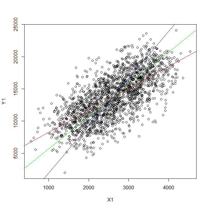
3. it lies between the two ordinary linear regression lines
4. it crosses them where they cross each other at the centroid of the observations, and
5. it is very easy to calculate.

The slope is the geometric mean of the slopes of the two ordinary linear regression slopes. It is also what you would get if you standardised the $x$ and $y$ observations, drew a line at 45° (or 135° if there is negative correlation) and then de-standardised the line. It could also be seen as equivalent to making an implicit assumption that the variances of the two sets of errors are proportional to the variances of the two sets of observations; as far as I can tell, you claim not to know which way this is wrong.

Here is some R code to illustrate: the red line in the chart is OLS regression of $Y$ on $X$, the blue line is OLS regression of $X$ on $Y$, and the green line is this simple method. Note that the slope should be about 5.

set.seed(2011)
X0 <- 1600:3600
Y0 <- 5*X0 + 700
X1 <- X0 + 400*rnorm(2001)
Y1 <- Y0 + 2000*rnorm(2001)
slopeOLSXY  <- lm(Y1 ~ X1)$coefficients[2]     #OLS slope of Y on X
slopeOLSYX  <- 1/lm(X1 ~ Y1)$coefficients[2]   #Inverse of OLS slope of X on Y
slopesimple <- sd(Y1)/sd(X1) *sign(cov(X1,Y1)) #Simple slope
c(slopeOLSXY, slopeOLSYX, slopesimple)         #Show the three slopes
# 3.408292 7.362876 5.009475 
c(slopeOLSXY/cor(X1,Y1), slopeOLSYX*cor(X1,Y1), slopesimple) # adjust for cor
# 5.009475 5.009475 5.009475 
plot(Y1~X1)
abline(mean(Y1) - slopeOLSXY  * mean(X1), slopeOLSXY,  col="red")
abline(mean(Y1) - slopeOLSYX  * mean(X1), slopeOLSYX,  col="blue")
abline(mean(Y1) - slopesimple * mean(X1), slopesimple, col="green")