If A is Poisson, you would speak of its rate of occurrence, rather than its probability.
If this is to be based on data, rather than a fully identified joint distribution, a simple approach is to condition on is observed values of B and the interest is if the observed counts of A tends to be higher when the count of B is higher.
So the question would be 'How would we see if the rate of occurrence of A increases when the occurrence of B is higher?'
If that's your intent, we can certainly get somewhere (if not, please edit your question to clarify your actual intent):
You might do something simple, like look for a positive correlation (not necessarily linear - you might look at monotonic association via something like a nonparametric correlation, perhaps).
Another approach would be to do a Poisson regression (GLM) of the counts of A on counts of B (hopefully including any other known or likely important covariates); in some other cases, B might be treated as an exposure by including an offset in a Poisson regression (but I don't think that would be suitable for this particular example).
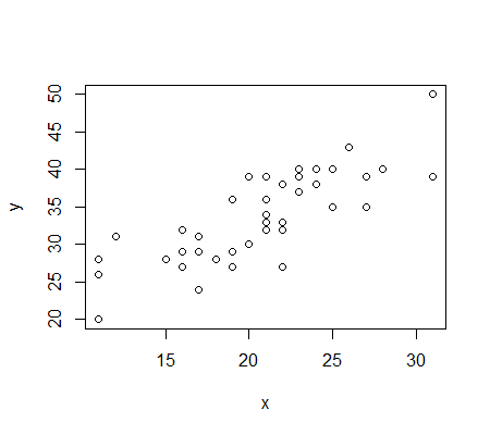
Here's an illustration with simulated data (in this case I know the model, because I created the data):

As we see from the plot, the two are positively associated. Their Pearson correlation is:
 cor(x,y)
[1] 0.8057106
Here I fit a GLM (in R) with identity link (more commonly, a log link would be used, but the model here is closer to the data generating model in this particular example). In this case, we fit $E(Y|X=x) = \beta_0+\beta_1 x$, which looks like a regression model, but with the GLM here the model takes account of the fact that the observations are conditionally Poisson. The command
summary(glm(y~x,family=poisson(link=identity)))
fits the model mentioned above, with output:
Coefficients:
            Estimate Std. Error z value Pr(>|z|)
(Intercept)  13.9571     3.6826    3.79 0.000151 ***
x             0.9533     0.1806    5.28 1.29e-07 ***
---
Signif. codes:  0 ‘***’ 0.001 ‘**’ 0.01 ‘*’ 0.05 ‘.’ 0.1 ‘ ’ 1

(Dispersion parameter for poisson family taken to be 1)

    Null deviance: 42.907  on 39  degrees of freedom
Residual deviance: 15.284  on 38  degrees of freedom
AIC: 232.81
In this case, the fitted model reproduces the actual process used to create it fairly well; the true model is that $x$ was generated from a conditionally Poisson model (with mean that took two different values), and $y$ was equal to $x$ plus a 'background' Poisson process (with constant intensity).
The interpretation here is that when $x$ increases by $1$, on average the $y$ count increases by about $0.95$
The intercept term picked up the background process (which had population mean 13), and the slope term picked up the $x$ effect (which had population coefficient 1).
As gung suggests below, if you take daily rainfall and daily hail as Bernoulli (rained or not, hailed or not, for each day), then you can deal with probability rather than counts, and there are a variety of ways to model that. His suggestions in comments are a good way of looking at the problem (quite a bit more sophisticated than my suggestions here), and would get you closer to conditioning on estimated underlying probability per unit time rather than directly observed rate per unit time.

