Sample from a custom continuous distribution in R

Question

I have a probability density function in R and I want to draw a single sample from it. How do I do that?

My current solution (and the one Google keeps giving me) is to evaluate the function for a dense set of values (x) giving the associated probabilities (px) and then draw a sample using sample(x, size=1, prob=px). Since I draw thousands of samples this way, simulating the distribution is really computationally heavy and is discrete even though it should be continuous.

Specifically, I'm writing my own Gibbs sampler to infer which means and standard deviations could have caused a vector of observations (bayesian inference). I sample from the distribution made up of likelihood * prior. Here's a minimal example of the loop-in-loop version I'm currently doing:

# values to assign posterior probabilities to. here 1000 values are used to simulate continuity.
mu.x = seq(from=0.001, to=20, length.out=1000)

# the likelihood distribution which will be called for varying mu and a fixed sigma and fixed D.
likelihoodMu =    function(mu, sigma, D) mu.likelihood = ((2 * pi * sigma^2) ^ (-length(D) / 2)) * exp(-1 / (2 * sigma^2) * sum((D - mu)^2))

# will collect samples
mySamples = rep(NA, length(mu.x))

# Draw 5000 samples
for(i in 1:5000) {
   # Loop over mu.x and get likelihood for each value
   mu.likelihoodDistribution = sapply(mu.x, likelihoodMu, sigma=2, D=c(1,2,3))

   # Draw a sample from the likelihood distribution calculated above
   mySample = sample(mu.x, size=1, prob=mu.likelihoodDistribution)
}

I'm looking for a way to sample directly from the likelihood function in R instead of going through the discrete and computationally heavy seq-sapply-sample simulation. In the example above, something like sample('mu', FUN=likelihoodMu, sigma=2, D=c(1,2,3), size=1) would be nice. It should preferably be general, as I'm sampling from different kinds of distributions.

Answer 1

If you want to sample from a certain pdf, you can use

rejection sampling which requires nothing more than the density function and the specification of a value as upper bound which is at least as large as the largest value of the density function. The disadvantage is that it can eventually be a very inefficient way to sample depending on the shape of the density function.

inverse transform sampling is the preferred way if the inverse of the distribution function is known. This is the case for the likelihood in your example since it is a Gaussian distribution and the associated quantile function (=inverse distribution function) is available in R. In general, inverse transform sampling works by sampling from a uniform distribution in the interval [0,1] and use the obtained values as the argument of the quantile function. The resulting values from the quantile function then follow the specified probability distribution.

To elaborate on the example: Since the likelihood is for a Gaussian distribution, it is maximized by setting $\mu$ to the arithmetic mean of the $D$ values $$\mu = \frac{1}{n}\sum_i^n D_i$$ from which the variance can be calculated by $$\text{Var}(\mu)=\frac{1}{n^2}\sum_i^n \text{Var}(D_i)=\frac{\sigma^2}{n}$$ Thus the $\mu$ value follows a Gaussian distribution $N(\mu,\sigma/\sqrt{n})$. Instead of implementing inverse transform sampling yourself, you could also use the rnorm function.

Answer 2

There are some posts on the internet about rejection sampling, but I found this one to be the most helpful. My example is from there, with minor modifications. If you need to speed things up a bit more, you could use data.table package which can make you feel dizzy from speed gains. I didn't bother because this particular implementation was instantaneous for me.

Here's my implementation of a function for $x \geq 0$.

kindaSortaLikeAcdfWeibullButNotReally <- function(x, sigma, b, mx) {
  exp(-(x/sigma)^(-b)) * mx
}

xrange <- 400 # function range from 0 (implicit) to x
N <- 100000 # number of samples
b <- -2.16
mx <- 35.48
sigma <-  147.17

xy <- data.frame(proposed = runif(N, min = 0, max = xrange))

xy$fit <- kindaSortaLikeAcdfWeibullButNotReally(x = xy$proposed, 
                                                sigma = sigma, b = b, mx = mx)
xy$random <- runif(N, min = 0, max = 1)

maxDens <- max(xy$fit)

xy$accepted <- with(xy, random <= fit/maxDens)
# retain only those values which are "below" the custom distribution
xy <- xy[xy$accepted, ]

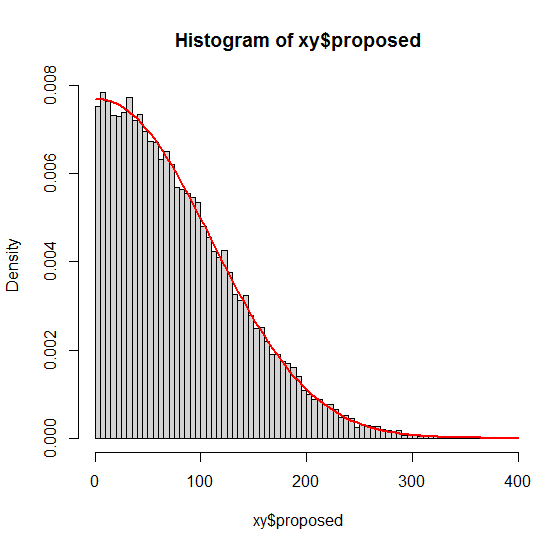
hist(xy$proposed, freq = FALSE, breaks = 100, col = "light grey")
# multiply by 130 to make it look fit nicely
curve(weibullLikeDistribution(x, sigma = sigma, b = b, mx = mx)/(maxDens * 130),
      from = 0, to = 400, add = TRUE, col = "red", lwd = 2)

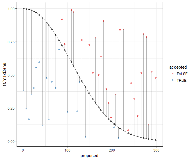
Here's an image which shows how the algorithm works. You find the distribution (fit, in black dots), throw a bunch of values in a square around the distribution (random column) and see if it's higher than the fit or not.

# modify above example to put 
mx <- 1
xrange <- 300
# xy <- xy[xy$accepted, ] # skip this step - you'll see why if you don't

library(ggplot2)

xys <- xy[order(xy$proposed), ]
xys <- xys[seq(1, nrow(xys), by = 11), ]

ggplot(xy, aes(x = proposed, y = fit/maxDens)) +
  theme_bw() +
  scale_color_brewer(palette = "Set1") +
  geom_line(alpha = 0.5) +
  geom_point(data = xys, aes(y = random, color = accepted), alpha = 0.5) +
  geom_point(data = xys, aes(x = proposed, y = fit/maxDens), alpha = 0.5) +
  geom_segment(data = xys, aes(x = proposed, y = random, xend = proposed, yend = fit/maxDens), alpha = 0.3)