23
$\begingroup$

Is there a (stronger?) alternative to the arcsin square root transformation for percentage/proportion data? In the data set I'm working on at the moment, marked heteroscedasticity remains after I apply this transformation, i.e. the plot of residuals vs. fitted values is still very much rhomboid.

Edited to respond to comments: the data are investment decisions by experimental participants who may invest 0-100% of an endowment in multiples of 10%. I have also looked at these data using ordinal logistic regression, but would like to see what a valid glm would produce. Plus I could see the answer being useful for future work, as arcsin square root seems to be used as a one-size-fits all solution in my field and I hadn't come across any alternatives being employed.

$\endgroup$
6
  • 2
    $\begingroup$ What are the fitted values from? What is your model? arcsin is (approximately) variance stabilising for binomial, but you will still have "edge" effects if the proportions are close to 0 or 1 - because the normal part effectively gets truncated. $\endgroup$ Commented May 19, 2011 at 14:49
  • 1
    $\begingroup$ Let me double down on what @probabilityislogic has said and also inquire about where the data come from. There might be something in the problem which suggests another transformation, or another model entirely, which might be more appropriate and/or interpretable. $\endgroup$
    – JMS
    Commented May 19, 2011 at 18:47
  • 1
    $\begingroup$ @prob @JMS Why don't we let the OP, who I believe is quite knowledgeable about stats, try the transformation route first? Then, if that doesn't work, it would be fruitful to commence a new thread in which the problem is presented less narrowly. Your comments would be appropriate in that context. $\endgroup$
    – whuber
    Commented May 19, 2011 at 19:08
  • 3
    $\begingroup$ There are huge problems with the arcsine square root transformation, described bluntly in the amusingly titled paper The arcsine is asinine: the analysis of proportions in ecology $\endgroup$
    – mkt
    Commented Sep 11, 2019 at 20:01
  • 2
    $\begingroup$ @mkt Thanks for the reference, this has gone straight into next term's lecture on generalised linear models. $\endgroup$ Commented Sep 13, 2019 at 8:45

2 Answers 2

34
$\begingroup$

Sure. John Tukey describes a family of (increasing, one-to-one) transformations in EDA. It is based on these ideas:

  1. To be able to extend the tails (towards 0 and 1) as controlled by a parameter.

  2. Nevertheless, to match the original (untransformed) values near the middle ($1/2$), which makes the transformation easier to interpret.

  3. To make the re-expression symmetric about $1/2.$ That is, if $p$ is re-expressed as $f(p)$, then $1-p$ will be re-expressed as $-f(p)$.

If you begin with any increasing monotonic function $g: (0,1) \to \mathbb{R}$ differentiable at $1/2$ you can adjust it to meet the second and third criteria: just define

$$f(p) = \frac{g(p) - g(1-p)}{2g'(1/2)}.$$

The numerator is explicitly symmetric (criterion $(3)$), because swapping $p$ with $1-p$ reverses the subtraction, thereby negating it. To see that $(2)$ is satisfied, note that the denominator is precisely the factor needed to make $f^\prime(1/2)=1.$ Recall that the derivative approximates the local behavior of a function with a linear function; a slope of $1=1:1$ thereby means that $f(p)\approx p$ (plus a constant $-1/2$) when $p$ is sufficiently close to $1/2.$ This is the sense in which the original values are "matched near the middle."

Tukey calls this the "folded" version of $g$. His family consists of the power and log transformations $g(p) = p^\lambda$ where, when $\lambda=0$, we consider $g(p) = \log(p)$.

Let's look at some examples. When $\lambda = 1/2$ we get the folded root, or "froot," $f(p) = \sqrt{1/2}\left(\sqrt{p} - \sqrt{1-p}\right)$. When $\lambda = 0$ we have the folded logarithm, or "flog," $f(p) = (\log(p) - \log(1-p))/4.$ Evidently this is just a constant multiple of the logit transformation, $\log(\frac{p}{1-p})$.
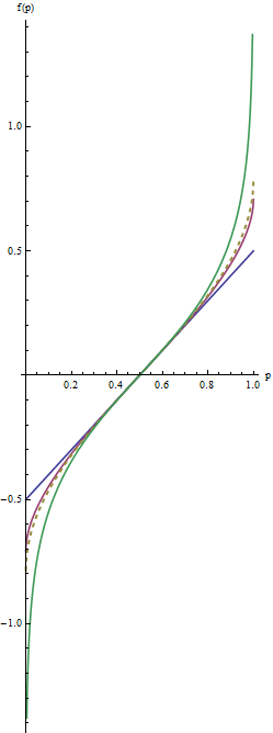
Graphs for lambda=1, 1/2, 0, and arcsin

In this graph the blue line corresponds to $\lambda=1$, the intermediate red line to $\lambda=1/2$, and the extreme green line to $\lambda=0$. The dashed gold line is the arcsine transformation, $\arcsin(2p-1)/2 = \arcsin(\sqrt{p}) - \arcsin(\sqrt{1/2})$. The "matching" of slopes (criterion $(2)$) causes all the graphs to coincide near $p=1/2.$

The most useful values of the parameter $\lambda$ lie between $1$ and $0$. (You can make the tails even heavier with negative values of $\lambda$, but this use is rare.) $\lambda=1$ doesn't do anything at all except recenter the values ($f(p) = p-1/2$). As $\lambda$ shrinks towards zero, the tails get pulled further towards $\pm \infty$. This satisfies criterion #1. Thus, by choosing an appropriate value of $\lambda$, you can control the "strength" of this re-expression in the tails.

$\endgroup$
4
  • $\begingroup$ whuber, know of any R function that does this one automatically? $\endgroup$
    – John
    Commented May 19, 2011 at 20:34
  • 1
    $\begingroup$ @John No I don't, but it's simple enough to implement. $\endgroup$
    – whuber
    Commented May 19, 2011 at 20:46
  • 2
    $\begingroup$ I didn't see it as basically difficult but it would be nice if there was something like the boxcox tranforms that automatically plot out the best selection for lambda. Yes, not terrible to implement... $\endgroup$
    – John
    Commented May 19, 2011 at 20:59
  • 2
    $\begingroup$ Thanks whuber, this is exactly the kind of thing I was looking for and the graph is really helpful. Definitely agree with John that something like the boxcox would be helpful, but this seems simple enough to work through. $\endgroup$ Commented May 20, 2011 at 11:01
7
$\begingroup$

One way to include is to include an indexed transformation. One general way is to use any symmetric (inverse) cumulative distribution function, so that $F(0)=0.5$ and $F(x)=1-F(-x)$. One example is the standard student t distribution, with $\nu$ degrees of freedom. The parameter $v$ controls how quickly the transformed variable wanders off to infinity. If you set $v=1$ then you have the arctan transform:

$$x=arctan\left(\frac{\pi[2p-1]}{2}\right)$$

This is much more extreme than arcsine, and more extreme than logit transform. Note that logit transform can be roughly approximated by using the t-distribution with $\nu\approx 8$. SO in some way it provides an approximate link between logit and probit ($\nu=\infty$) transforms, and an extension of them to more extreme transformations.

The problem with these transforms is that they give $\pm\infty$ when the observed proportion is equal to $1$ or $0$. So you need to somehow shrink these somehow - the simplest way being to add $+1$ "successes" and $+1$ "failures".

$\endgroup$
5
  • 2
    $\begingroup$ For various reasons, Tukey recommends adding +1/6 to counts. Note that this reply is a special case of Tukey's folding approach that I described: any CDF with positive PDF is monotonic; folding a symmetric CDF leaves it unchanged. $\endgroup$
    – whuber
    Commented May 20, 2011 at 13:19
  • 2
    $\begingroup$ I have been wondering where your rough approximation comes from. How do you arrive at $\nu\approx 8$? I can't reproduce this. I accept that the approximation must break down at the extremes of $p$ near $0$ or $1$, but I find that $\nu=5$ is a much better match for the logit for $p$ near $1/2$. Are you perhaps optimizing some measure of an average difference between the CDF of $t_\nu$ and $\text{logit}$? $\endgroup$
    – whuber
    Commented Oct 17, 2011 at 13:27
  • 2
    $\begingroup$ @whuber - you give me too much credit. My suggestion was based on looking at a graph of the pdf of $t_8$, a graph of the logistic pdf $f(x)=e^{-x}(1+e^{-x})^{-2}$, and a graph of standard normal pdf. $5$ degrees of freedom matches the excess kurtosis, and may well be better. $\endgroup$ Commented Oct 18, 2011 at 1:09
  • 5
    $\begingroup$ @whuber One reason for adding 1/6 to counts is that the resulting "started" count approximates the median posterior assuming a binomial distribution with Jeffreys prior (I write a little bit about this here: sumsar.net/blog/2013/09/a-bayesian-twist-on-tukeys-flogs). However I don't know if this was Tukey's reason for adding 1/6. Do you know what his reason might have been? $\endgroup$ Commented Apr 28, 2015 at 13:19
  • 4
    $\begingroup$ @Rasmuth In EDA, p. 496, Tukey writes "The [usage] we here recommend does have an excuse, but since this excuse (i) is indirect and (ii) involves more sophisticated considerations, we shall say no more about it. What we recommend is adding 1/6 to all split counts, thus 'starting' them." (A "split count" of any value $x$ is the number of $x_i\lt x$ plus half the number of $x_i=x$ in a batch of data $(x_i)$.) I don't recall coming across these "sophisticated considerations" in other Tukey papers or books I have read, but always imagined they might be related to probability plotting points. $\endgroup$
    – whuber
    Commented Apr 28, 2015 at 14:25

Your Answer

By clicking “Post Your Answer”, you agree to our terms of service and acknowledge you have read our privacy policy.

Not the answer you're looking for? Browse other questions tagged or ask your own question.