GRS statistic in R to test that intercepts from multivariate panel regression are jointly zero?

Question

The GRS statistic is the Gibbons et al. (1989) statistic that tests whether the estimated intercepts from a multiple regression model are jointly zero.

The typical scenario involves a multivariate linear panel regression where you are explaining the returns to securities in terms of its exposures to factor return series. Theoretically, a good factor model will have an intercept statistically indistinguishable from zero.

How do I calculate the GRS statistic in R?

Thank you

Answer 1

As stated in the GRS paper, you have to estimate the intercepts of each asset in your portfolio by sample OLS. This will give you a vector of estimates $\hat{\alpha}_1, \hat{\alpha}_2, \ldots$. Put these into a vector $\hat{\alpha}$. Now estimate the covariance matrix of the assets in the 'usual' way, calling it $\hat{\Sigma}$. Then compute $W_u = \hat{\alpha}^{\top} \hat{\Sigma}^{-1} \hat{\alpha} / (1 + \hat{\theta}^2),$ where $\hat{\theta}$ is the sample-estimated Sharpe ratio of the market portfolio (the one that you used in the individual OLS regressions as the market). Then $T W_u$ should follow a Hotelling Law, where $T$ is the number of days observed (for the regressions. Note that a modification of the GRS test allows one to use a covariance esimator built on different data from the OLS regressions).

The test statistic is then computed as below:

#compute the sample Sharpe ratio
sample.sr <- function(x) {
    mu <- mean(x)
    sg <- sd(x)
    return(mu / sg)
}

#srets is a T x N matrix of the returns of the assets
# by return, I mean the relative return (V_t / V_{t-1}) - 1,
# where V_t is the 'value' of the asset at time t.
# relative returns make more sense when combined 'laterally'
#mret is a T-vector of the returns of the 'market'
GRS.test <- function(srets,mret) {
    T <- dim(srets)[1]
    N <- dim(srets)[2]

    #this is 'good' R style, but probably slow as hell.
    #would be faster to precompute the solution to the
    #normal equations and apply it en masse to the srets
    #matrix ... 
    reg.func <- function (y, m) {
        mod <- lm(y ~ m)
        mod$coefficients["(Intercept)"]
    }
    alphas <- as.vector(apply(srets, 2, reg.func, mret))

    #now the sigma hat;
    Sig.hat <- cov(srets)
    mkt.sr <- sample.sr(mret)

    #the GRS test statistic
    W.u <- t(alphas) %*% solve(Sig.hat,(alphas)) / (1 + mkt.sr^2)

    #convert to F
    F.stat <- T * (T - N - 1) * W.u / (N * (T - 2))
    p.val <- pf(F.stat, N, T-N-1, 0, lower.tail = FALSE)

    return(list('Wu' = W.u,'Fstat' = F.stat,'pval' = p.val))
}

#generate population data under the null to test the code;
#return the p-value for the data
GRS.gen.null <- function(T,N) {
    srets <- matrix(rnorm(T*N),ncol=N)
    mret <- as.vector(rnorm(T))
    test.it <- GRS.test(srets,mret)
    return(test.it$pval)
}

#always test your code under the null!
set.seed(1066)

nday <- 150            #'T'
nstock <- 8            #'N'
ntrial <- 2048         #number of experiments

should.be.p <- replicate(ntrial,GRS.gen.null(nday,nstock))
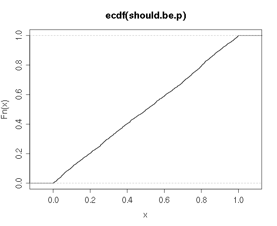
plot(ecdf(should.be.p))

I tested the function under the null hypothesis to confirm uniformity of the resultant p-values. Here is a plot:

This is a brain dead form of the null, where the stocks have no beta as well as no alpha (I was in a hurry). Probably one would want to test the power as well. Also note that using the some matrix math instead of calling lm will probably speed up this code quite a bit.

You can also use the F distribution to compute confidence intervals on the non-centrality parameter (assumed to be zero under the null).

If there is not a stock R package for performing this test, I would be very surprised (and would like to write such a package in that case ... )

Answer 2

The GRS test assumes returns are homoscedastic with no auto-correlation. For a robust test, using GMM is recommended (see Cochrane's Asset Pricing p230-235). This can be easily implemented using the gmm package. The package's vignette (section 3.5) provides an example for testing the CAPM using time-series regression. This is the GRS test (assuming one factor that's the market) except a GMM approach is additionally robust to heteroscedasticity and auto-correlation. Here's the example code (using the Finance dataset in the gmm package and also invoking linearHypothesis() in the car package):

data(Finance) # load data
r <- Finance[1:500,1:5]
rm <- Finance[1:500,"rm"]
rf <- Finance[1:500,"rf"]

z <- as.matrix(r-rf)
zm <- as.matrix(rm-rf)
res <- gmm(z~zm,x=zm) # use gmm 

R <- cbind(diag(5),matrix(0,5,5)) # conduct test for the intercepts only and not the betas (in this example there are 5 test assets)
c <- rep(0,5) # test that all 5 intercepts equal 0
linearHypothesis(res,R,c,test = "Chisq") # perform test