ETS() function, how to avoid forecast not in line with historical data?

Question

I am working on an alogorithm in R to automatize a monthly forecast calculation. I am using, among others, the ets() function from the forecast package to calculate forecast. It is working very well.

Unfortunately, for some specific time series, the result I get is weird.

Please, find below the code i am using :

train_ts<- ts(values, frequency=12)
fit2<-ets(train_ts, model="ZZZ", damped=TRUE, alpha=NULL, beta=NULL, gamma=NULL, 
            phi=NULL, additive.only=FALSE, lambda=TRUE, 
            lower=c(0.0001,0.0001,0.0001,0.8),upper=c(0.9999,0.9999,0.9999,0.98), 
            opt.crit=c("lik","amse","mse","sigma","mae"), nmse=3, 
            bounds=c("both","usual","admissible"), ic=c("aicc","aic","bic"),
            restrict=TRUE)  
ets <- forecast(fit2,h=forecasthorizon,method ='ets')   

Please, you will find below the concerned history data set :

 values <- c(27, 27, 7, 24, 39, 40, 24, 45, 36, 37, 31, 47, 16, 24, 6, 21, 
35, 36, 21, 40, 32, 33, 27, 42, 14, 21, 5, 19, 31, 32, 19, 36, 
29, 29, 24, 42, 15, 24, 21)

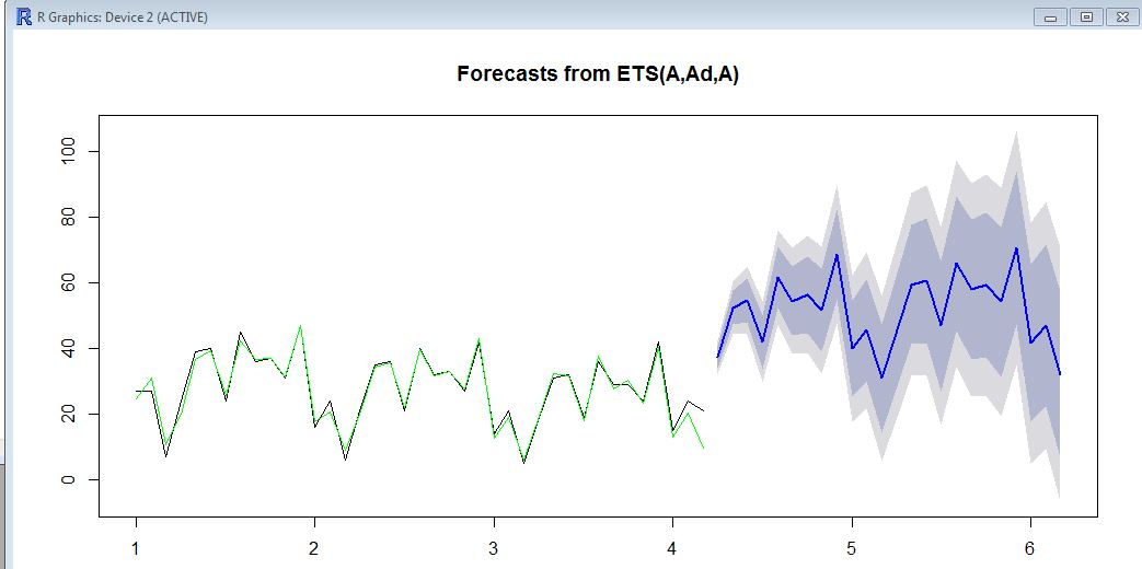
Here, on the graph, you will see the historical data (black), the fitted value (green) and the forecast(blue). The forecast is definitely not in lines with the fitted value.

Do you have any idea on how to "bound" the forecat to be "in line" with the historical sales?

Answer 1

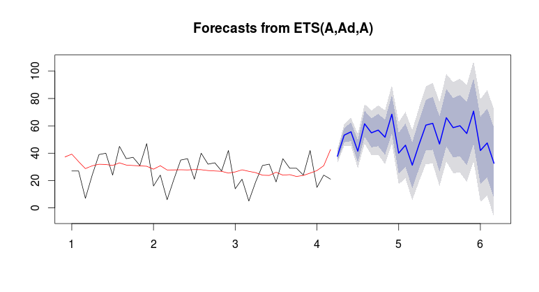
As @forecaster has pointed out, this is caused by outliers at the end of the series. You can see the problem clearly if you plot the estimated level component over the top:

plot(forecast(fit2))
lines(fit2$states[,1],col='red')

Note the increase in the level at the end of the series.

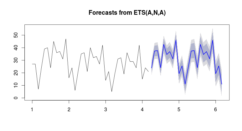
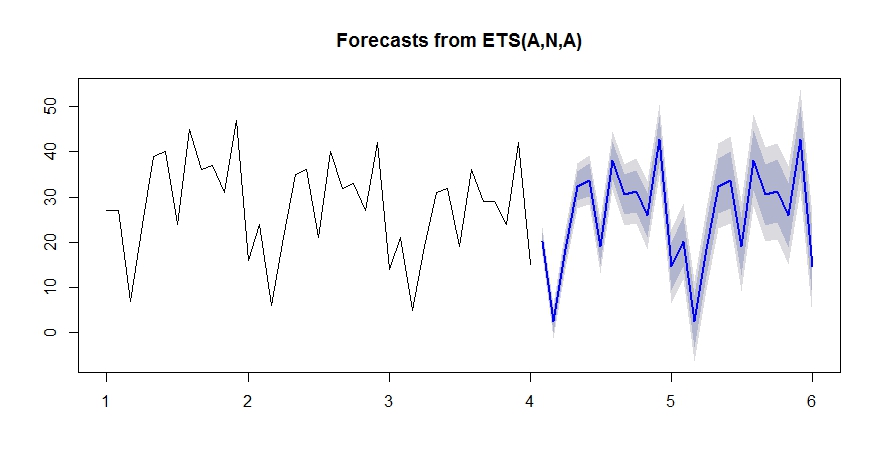
One way to make the model more robust to outliers is to reduce the parameter space so that the smoothing parameters must take smaller values:

fit2 <- ets(train_ts, upper=c(0.3,0.2,0.2,0.98))  
plot(forecast(fit2))

Answer 2

This is textbook case of having outliers at the end of the series and its unintended consequences. The problem with your data is that the last two points are outliers, you might want to identify and treat outliers before you run the forecasting algorithms. I'll update my answer and analysis later today on some strategies to identify outliers. Below is the quick update.

When I rerun ets with last two data points removed, I get a reasonable forecast. Please see below:

values.clean <- c(27, 27, 7, 24, 39, 40, 24, 45, 36, 37, 31, 47, 16, 24, 6, 21, 
                  35, 36, 21, 40, 32, 33, 27, 42, 14, 21, 5, 19, 31, 32, 19, 36, 
                  29, 29, 24, 42, 15)## Last two points removed

train_ts.clean<- ts(values.clean, frequency=12)
fit2.clean<-ets(train_ts.clean)  
ets.f.clean <- forecast(fit2.clean,h=24)
plot(ets.f.clean)

Answer 3

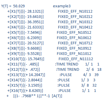
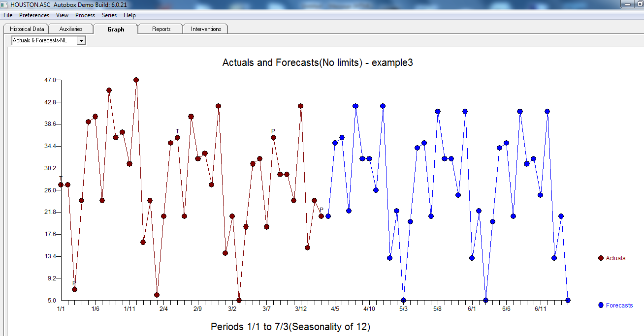
@forecaster you are correct that the last value is an outlier BUT periood 38 (the penultimate value) is not an outlier when you take into account trends and seasonal activity. This is a defining/teaching moment for testing/evaluating alternative robust approaches. If you don't identify and adjust for anomalies then the variance is inflated causing other items to not be found. Period 32 is also an outlier. Periods 3,32 and 1 are also outliers. There is a statistically significant trend in the series for the first 17 values but abates thereafter starting at period 18. So, there are really two trends in the data. The lesson to be learned here is that simple approaches that assume no trend or a particular form of a trend and/or tacitly assumes a specific form of the auto-regressive process need to be seriously questioned. Going forward a good forecast should have to consider the possible continuation of the exceptional activity found at the ultimate point (period 39). It is impossible to extract this from the data.

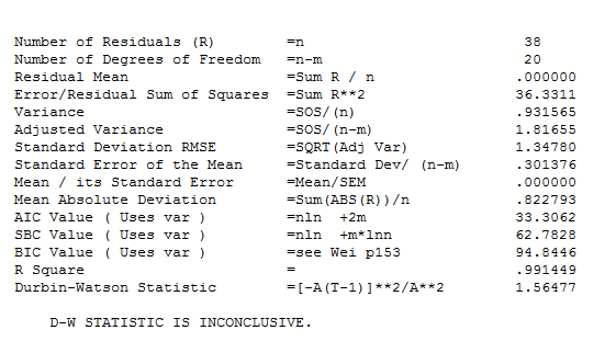
This is a possibly useful model:

The final model's statistics are here The Actual/Fit and Forecast graph is interesting as it highlights the exceptional activity.