1
$\begingroup$

I've got data points from a simulation as coordinates in a text-files like so:

23 0.000022842
24 0.000022842
25 0.000091368
26 0.000251262
27 0.000182736
28 0.000411156
29 0.000890838
30 0.00143905
31 0.00246694
32 0.00317504
33 0.0042943
34 0.00719523
35 0.00922817
36 0.0134083
37 0.0150072
38 0.019233
39 0.0228877
40 0.0281642
41 0.0320702
42 0.0350168
43 0.038306
44 0.0418694
45 0.0433541
46 0.0468946
47 0.0458896
48 0.0487905
49 0.0500925
50 0.045113
51 0.0458667
52 0.0423034
53 0.0418009
54 0.0369355
55 0.0349254
56 0.0311565
57 0.0294205
58 0.026314
59 0.0237557
60 0.0213344
61 0.017931
62 0.0151899
63 0.0135453
64 0.0115352
65 0.00918248
66 0.00778912
67 0.00669271
68 0.00532219
69 0.00479682
70 0.00395167
71 0.00322072
72 0.00262683
73 0.00187304
74 0.00121063
75 0.0011421
76 0.00111926
77 0.000708102
78 0.000708102
79 0.000479682
80 0.000319788
81 0.000205578
82 0.000251262
83 0.000137052
84 0.000091368
85 0.000091368
86 0.00011421
87 0.000045684
88 0.000045684
92 0.000045684
94 0.000045684

with 1st column being my x-data and 2nd column being probability values, accordingly.

The probability density function of this data first looked like a binomial distribution to me so I plotted an approximated binomial pdf that in the end didn't really match the simulated data.

The plot has got a relatively slight right heavy tail, so I'm wondering which distribution description would return the best regression curve in python.

I've already tried a polynomial fit but then there's the problem with the oscillating edges - Note: I will use the regression function in order to sum up values from k to infinity, so what I actually need is a smooth fit for the edges and a tool that returns the function I need.

I'd appreciate approaches with python and bash!

$\endgroup$
8
  • $\begingroup$ Could you explain what you mean by "edges" and "sum up values ... to infinity", given your data stop at $x=94$, which seems just a little short of $\infty$? Are your "probability values" actually relative frequencies? (They look like counts divided by $43779$.) If so, they are best analyzed in terms of the counts themselves. Please note that this is not a regression problem: it's a distribution estimation problem. Using regression techniques is likely to go awry. $\endgroup$
    – whuber
    Commented Aug 26, 2015 at 13:56
  • $\begingroup$ @whuber: Thanks for your response! 1) By edges I mean values close to 23 and 94 - I think this is called the RUNGE PROBLEM; 2) Yes, my probability values are actually relative frequencies.; 3) And by sum up, I'm referring to a currently unknown function that fits my data and that I can use for calculations such as a summation from a value k=26 to ∞.; Thanks for the valuable hint of 'distribution estimation'! - What do you mean by '... analyzed in terms of the counts themselves', would you please explain? - I'm really desperate ... $\endgroup$ Commented Aug 26, 2015 at 14:02
  • $\begingroup$ ... since I'm not very familiar with tools I could use to proceed with my calculations and for calculations I need an estimated function :/ $\endgroup$ Commented Aug 26, 2015 at 14:05
  • $\begingroup$ Your data will exhibit "oscillating edges" because the relative uncertainty is greater for any low count than for a higher count. An accurate fitting procedure will take this into account. That's routine. Your special problem concerns a gross extrapolation beyond what you have actually observed: the summation to infinity. There's nothing in these data that give any direct information about that sum. To make progress, you have to adopt an assumption--either explicitly or implicitly--about the distribution of the frequencies for higher values of $x$. $\endgroup$
    – whuber
    Commented Aug 26, 2015 at 14:09
  • $\begingroup$ My assumption was a binomial distribution but it doesn't really 'represent' my data. Would you kindly give me a hint for an appropriate assumption? $\endgroup$ Commented Aug 26, 2015 at 14:18

1 Answer 1

1
$\begingroup$

I would suggest that you go back to the original data and use methods like those posted here to find the best fitting distribution.

My apologies for not writing Python code. I do not use Python as a development tool. I rescaled the data to be the counting numbers from which it was apparently obtained and wrote the following Mathematica code

(begin code)

x = {23, 24, 25, 26, 27, 28, 29, 30, 31, 32, 33, 34, 35, 36, 37, 38, 39, 40, 41, 42, 43, 44, 45, 46, 47, 48, 49, 50, 51, 52, 53, 54, 55, 56, 57, 58, 59, 60, 61, 62, 63, 64, 65, 66, 67, 68, 69, 70, 71, 72, 73, 74, 75, 76, 77, 78, 79, 80, 81, 82, 83, 84, 85, 86, 87, 88, 92, 94};

y = {1, 1, 4, 11, 8, 18, 39, 63, 108, 139, 188, 315, 404, 587, 657, 842, 1002, 1233, 1404, 1533, 1677, 1833, 1898, 2053, 2009, 2136, 2193, 1975, 2008, 1852, 1830, 1617, 1529, 1364, 1288, 1152, 1040, 934, 785, 665, 593, 505, 402, 341, 293, 233, 210, 173, 141, 115, 82, 53, 50, 49, 31, 31, 21, 14, 9, 11, 6, 4, 4, 5, 2, 2, 2, 2};

s =.; m =.;

model = s m^x Exp[-m]/x!;

H = NMinimize[{Norm[y - model]}, {{s, 20000, 100000}, {m, 40, 60}}]

s = H[[2, 1, 2]];

m = H[[2, 2, 2]];

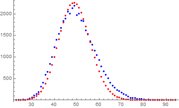
Show[ListPlot[Transpose[{x, y}], PlotStyle -> {Blue}], ListPlot[Table[{t, s m^t Exp[-m]/t!}, {t, 23, 94, 1}], PlotStyle -> {Red}]]

y - model

(end code)

The results are not quite Poisson.

{1050.39, {s -> 39747.1, m -> 49.1786}}

Blue for data, red for Poisson fit

Blue for data, red for Poisson

Hope that helps.

$\endgroup$

Your Answer

By clicking “Post Your Answer”, you agree to our terms of service and acknowledge you have read our privacy policy.

Not the answer you're looking for? Browse other questions tagged or ask your own question.