Inference on $P\left(\left.\sum_{i=1}^{N}X_{i}\ \right|\ \sum_{i=1}^{N}X_{i}^{2}\right)$ when $X_{i}\sim\mathcal{N}\left(0,1\right)$?

Question

Let:

$$X_{i}\overset{i.i.d}{\sim}\mathcal{N}\left(0,1\right)$$

Hence:

$$\sum_{i=1}^{N}X_{i}\sim\mathcal{N}\left(0,N\right)$$

and

$$\sum_{i=1}^{N}X_{i}^{2}\sim\chi^{2}\left(N\right)$$

What can be said about the following distribution:

$$P\left(\left.\sum_{i=1}^{N}X_{i}\ \right|\ \sum_{i=1}^{N}X_{i}^{2}\right)\quad ?$$

That is, I observe the sum of squared $X$'s and want to do inference on the sum of $X$'s. The fact that $f\left(x\right)=x^{2}$ is not injective makes it complicated.

So basically what I am asking is:

1. Can I get an analytical expression for $P\left(\left.\sum_{i=1}^{N}X_{i}\ \right|\ \sum_{i=1}^{N}X_{i}^{2}\right)$?
2. Can I evaluate $P\left(\left.\sum_{i=1}^{N}X_{i}\ \right|\ \sum_{i=1}^{N}X_{i}^{2}\right)$?
3. Do I know something about the moments of $P\left(\left.\sum_{i=1}^{N}X_{i}\ \right|\ \sum_{i=1}^{N}X_{i}^{2}\right)$ or anything else?

Answer 1

$Y^2 = \sum X_i^2$ is invariant under rotations. Therefore $(X_1/Y, \ldots, X_n/Y)$ is uniformly distributed on the unit sphere. Consequently the distribution of any linear combination

$$a_1 X_1 + a_2 X_2 + \cdots + a_n X_n = a Y \left(\frac{a_1}{a}\frac{X_1}{Y} + \cdots + \frac{a_n}{a}\frac{X_n}{Y}\right) = a Y Z,$$

with $a^2 = a_1^2 + a_2^2 + \cdots + a_n^2$, is the same as the distribution of any other linear combination with the same value of $aY$. For convenience, take $a_1=a_2=\cdots=a_{n-1}=0$ and $a_n=1$. To find the distribution of $Z$, we must therefore study the distribution of $X_n$ given that $(X_1,\ldots, X_n)$ lies on the unit sphere $S^{n-1}$ in $\mathbb{R}^n$.

The density between $X_n = h$ and $X_n = h+dh$ will be proportional to the volume of the infinitesimal band on $S^{n-1}$ between heights $h$ and $h+dh$. This band is a frustum of a circular cone with radii ranging from $(1-h^2)^{1/2}$ to $(1 - (h+dh)^2)^{1/2}$. It therefore has an $n-1$-dimensional content proportional to

$$f(h) = \frac{dh}{(1-h^2)^{1/2}}((1-h^2)^{1/2})^{n-2} + O(dh^2).$$

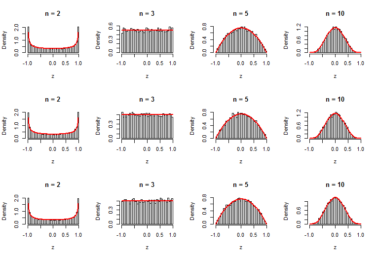
This is recognizable as a Beta$((n-1)/2, (n-1)/2)$ density that has been recentered at $0$ and scaled to be supported on $[-1,1]$. Consequently, $\sum X_i$ itself is $aY$ times that distribution.

---

Simulations in R bear out this result. For each of several values of $n$, a vector $a$ was randomly generated and then $10,000$ independent realizations of $\sum_{i=1}^n a_i X_i$ were created. For each of these, $Z$ was computed and summarized with a histogram. Over these histograms are drawn the claimed density function (of the rescaled, recentered Beta distribution). The agreement is excellent.

N <- 1e4
par(mfcol=c(3, 4))
for (n in c(2, 3, 5, 10)) {
  for (i in 1:3) {
    a <- rnorm(n)
    x <- matrix(rnorm(n*N), n, N)
    y <- apply(x, 2, function(y) sqrt(sum(y^2)))
    z <- ((a / sqrt(sum(a^2))) %*% x) / y

    hist(z, freq=FALSE, breaks=seq(-1,1,length.out=41), main=paste("n =", n))
    curve((1-x^2)^((n-3)/2)/(2^(n-2) * beta((n-1)/2, (n-1)/2)), col="Red", lwd=2, add=TRUE)
  }
}

Answer 2

I see @whuber beat me to the punch, but for posterity... You should be able to obtain an analyical expression this pretty easily using Bayes Law.

1) You already have $P\left( \sum_i X_i = Y \right)$

2) You should be able to calculate $P\left( \sum_i X_i^2 = Z \right)$. This is an integral over a spherical shell, which may seem daunting, but luckily the density is constant on that shell, so it should be the area of that shell times the density.

3) $P\left( \mathbf{X} | \sum_i X_i = Y \right)$ is a "slice" of a multivariate normal distribution by a hyperplane and is therefore another multivariate normal distribution. Similarly to in (2) you can then compute $P\left( \sum_i X_i^2 = Z | \sum_i X_i = Y \right)$.

So if "the frustum of a circular cone" scares you off, try answering (1), (2), and (3).