Is it appropriate to report standard error obtained by bootstrap when observed statistics is away from the median of the bootstrapped distribution?

Question

I quantified a statistics that measure the percentage of covariation between set of variables, lets say Int, across 3 groups (for each group Int was calculated). Int ranges from 0 to 100.

Afterwards I used bootstrap in order to obtain some measure of variability of the Int within each group (resampling was with replacement within each group).

Because I can not pass all the data and complex cod for the Int, below I generated (mimic) the pattern of the results that I obtained after bootstrap:

  set.seed (50)

# here "Int.boot.dist" mimic bootstrap distribution that I obtained
  Int.boot.dist <- rnorm (n = 100, mean = 50, sd = 15)

# boxplot     
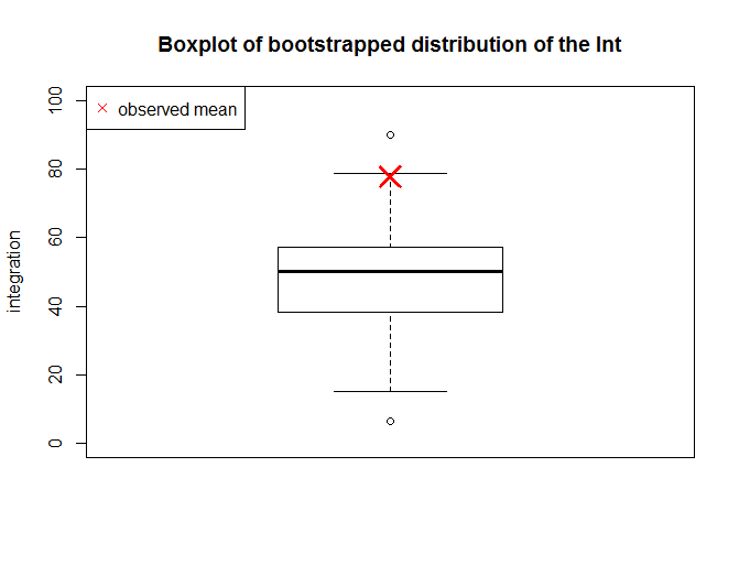
  boxplot (Int.boot.dist, main = "Boxplot of bootstrapped distribution of the Int", 
  ylab = "integration", ylim = c (0, 100))

# mimic observed mean
  obs.mean <- sample [order (sample, decreasing = T)][3]

  points (obs.mean, cex = 2.5, lwd = 3, pch = 4, col = "red")
  legend ("topleft", legend = "observed mean", cex = 1, col = "red", pch = 4)

As you can note, observed Int is almost like outlier and considerably far away from bootstrapped mean or median.

   ## plot (as a bar where height correspond to the observed Int) along with standard error    

           plot (Int.boot.dist, type = "n", xlim = c(0, 2), ylim = c (0, 100), 
               xlab =  "group1", ylab = "integration")
            x <- c (0.5, 1.5, 1.5, 0.5)
            y <- c (0, 0, obs.mean, obs.mean)
            polygon (x, y, border = "black", col = "gray")

    ## calculate standard error
    sd <- sqrt(var(sample))
            y0 <- obs.mean-sd
            y1 <- obs.mean+sd

            segments (1, y0, 1, y1, col = "red", lwd = 2)
            legend ("topleft", legend = "SDM", lwd = 2, col = "red")

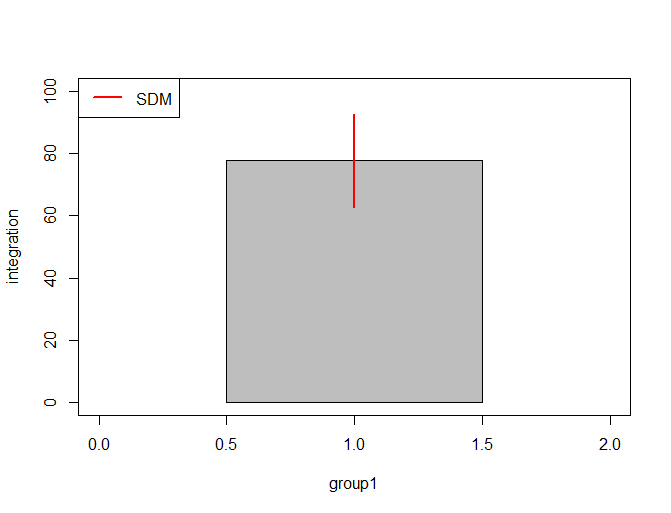
Second graph shows bar that corresponds to the observed Int value and red line shows standard error obtained by bootstrap.

Q1: Is it appropriate to report standard error (e.g. second graph) when observed statistics depart from mean or median of bootstrapped distribution?

Q2: What does such pattern tell us about the data and is it appropriate to compare such statistics at all?

Answer 1

You have demonstrated that your estimator for Int is probably biased; that is, the expected value of repeated sample estimates of Int is different from the population value of Int. The bootstrap was originally devised in part as a way to estimate such bias. Also, note that with your Int scale limited to 100 as a top value, there is no way for your Int values to have a normal distribution and that your confidence intervals are unlikely to be symmetric about the center value.

You don't specify how you calculate Int or the nature of the underlying data, but you should know that the standard Pearson correlation coefficient is a biased estimate of the population correlation coefficient even in the idealized case of variables having a bivariate normal distribution. So it's not surprising that your sample estimate of Int, which seems to have some sort of relation to a correlation coefficient, is also biased.

You should take advantage of already developed tools to solve your problem. The boot.ci function in the R boot package provides several types of estimates of confidence intervals. For your situation, with a biased estimator and a necessarily skewed distribution of your Int values (as they can't exceed 100), you would want to use the "bca" type of confidence interval. This Cross Validated Page goes into more detail about bootstrapping, with links to further information.