Likelihood ratio vs. score vs. Wald test: Different p values, which to use?

Question

From what I've been reading, amongst others on the site of the UCLA statistics consulting group likelihood ratio tests and Wald tests are pretty similar in testing whether two glm models show a significant difference in the fit for a dataset (excuse me if my wording might be a bit off). In essence I can compare two models and test if the second model shows a significantly better fit than the first, or there is no difference between the models. So the LR and Wald tests should show the same ballpark p-values for the same regression models. At least the same conclusion should come out.

Now I did both tests for the same model in R and get widely differing results. Here are results from R for one model:

lrtest(glm(data$y ~ 1), glm(data$y ~ 
 data$site_name, family="poisson"))
Likelihood ratio test

Model 1: data$y ~ 1
Model 2: data$y ~ data$site_name
  #Df  LogLik Df  Chisq Pr(>Chisq)    
1   2 -89.808                         
2   9 -31.625  7 116.37  < 2.2e-16 ***
---
Signif. codes:  0 ‘***’ 0.001 ‘**’ 0.01 ‘*’ 0.05 ‘.’ 0.1 ‘ ’ 1   

 lrtest(glm(data$y ~ 1, family="poisson"), 
  glm(data$y ~ data$site_name, family="poisson"))
Likelihood ratio test

Model 1: data$y ~ 1
Model 2: data$y ~ data$site_name
  #Df  LogLik Df  Chisq Pr(>Chisq)    
1   1 -54.959                         
2   9 -31.625  8 46.667  1.774e-07 ***
---
Signif. codes:  0 ‘***’ 0.001 ‘**’ 0.01 ‘*’ 0.05 ‘.’ 0.1 ‘ ’ 1 

 waldtest(glm(data$y ~ data$site_name, 
  family="poisson"))
Wald test

Model 1: data$y ~ data$site_name
Model 2: data$y ~ 1
  Res.Df Df      F Pr(>F)
1     45                 
2     53 -8 0.7398 0.6562   

 waldtest(glm(data$y ~ 1, family="poisson"), 
 glm(data$y~data$site_name, family="poisson")) 

Wald test

Model 1: data$y ~ 1
Model 2: data$y ~ data$site_name
  Res.Df Df      F Pr(>F)
1     53                 
2     45  8 0.7398 0.6562

About the data, data\$y contains count data and data\$site_name is a factor with 9 levels. There are 54 values in data\$y, with 6 values per level of data\$site_name.

Here are frequency distributions:

table(data$y)

 0  2  4  5  7 
50  1  1  1  1 
table(data$y, data$site_name)
   
    Andulay Antulang Basak Dauin Poblacion District 1 Guinsuan Kookoo's Nest Lutoban Pier Lutoban South Malatapay Pier
  0       6        6     6                          4        6             6            6             5              5
  2       0        0     0                          0        0             0            0             1              0
  4       0        0     0                          1        0             0            0             0              0
  5       0        0     0                          0        0             0            0             0              1
  7       0        0     0                          1        0             0            0             0              0

Now this data doesn't fit the Poisson distribution very well due to the enormous over-dispersion of zero counts. But with another model, where data\$y>0 fits the Poisson model quite well, and while using a zero-inflated Poisson model, I still get highly different Wald test and lrtest results. There the Wald test shows a p-value of 0.03 while the lrtest has a p-value 0.0003. Still a factor 100 difference, even though the conclusion might be the same.

So what am I understanding incorrectly here with the likelihood ratio vs Wald test?

Answer 1

It's important to note that although the likelihood ratio test and the Wald test are used by researchers to accomplish the same empirical goal(s), they are testing different hypotheses. The likelihood ratio test evaluates whether the data were likely to have come from a more complex model, vs. a more simple model. Put another way, does the addition of a particular effect allow the model to account for more information. The Wald test, conversely, evaluates whether it is likely that the estimated effect could be zero. It's a nuanced difference, to be sure, but an important conceptual difference nonetheless.

Agresti (2007) contrasts likelihood ratio testing, Wald testing, and a third method called the "score test" (he hardly elaborates on this test further). From his book (p. 13):

When the sample size is small to moderate, the Wald test is the least reliable of the three tests. We should not trust it for such a small n as in this example (n = 10). Likelihood-ratio inference and score-test based inference are better in terms of actual error probabilities coming close to matching nominal levels. A marked divergence in the values of the three statistics indicates that the distribution of the ML estimator may be far from normality. In that case, small-sample methods are more appropriate than large-sample methods.

Looking at your data and output, it seems that you do indeed have a relatively small sample, and therefore may want to place greater stock in the likelihood ratio test results vs. the Wald test results.

References

Agresti, A. (2007). An introduction to categorical data analysis (2nd edition). Hoboken, NJ: John Wiley & Sons.

Answer 2

First, I disagree somewhat with jsakaluk's answer that the two tests are testing different things - they are both testing whether the coefficient in the larger model is zero. They are just testing this hypothesis by making different approximations (see article linked to below).

Regarding the differences between their results, as jsakaluk said, this is likely due to the small sample size / that the log likelihood is far from quadratic. I wrote a blog post back in 2014 which goes through this for a simple binomial model, which may help further: http://thestatsgeek.com/2014/02/08/wald-vs-likelihood-ratio-test/

Answer 3

The disparity between Wald and likelihood-ratio test statistics arises from parameters at boundaries that signal complete separation problems in discrete choice models. In your frequency table, many sites have zero-only counts. Their corresponding coefficients in a Poisson regression approach negative infinity. In practice, the estimates might range somewhere -5 to -30, suggesting an incident-rate ratio of 1:148 to 1:1.06e+13. This challenges an accurate estimation, which is represented by huge standard errors. Score and likelihood-ratio tests are more reliable than Wald tests in such cases. Wald, score and likelihood-ratio tests are all designed to answer the same question on parameter significance because they address the same two-sided null hypothesis about model coefficients by comparing two nested models. The most common scenario is that only one coefficient is of interest and the reference value is zero, H0: β = 0 vs. H1: β != 0.

Solutions β for likelihood equations ∂ln⁡L ⁄ ∂β = 0 given y and x are maximum likelihood estimates. The observed information or negative Hessian matrix, (∂^2 ln⁡L)⁄(∂β∂β), which may not equal the expected Fisher information matrix in Poisson models, measures the curvature of ln⁡L and gives the asymptotic covariance matrix and standard errors of coefficients when inversed and evaluated at β (Greene & Hensher, 2010).

In addition to the condition number and positive definiteness of the Hessian matrix, behavior of the Wald test statistic, which is the squared ratio between a point estimate and its standard error, is another vehicle to examine convergence properties. For one coefficient β, the ratio β ⁄ se⁡β asymptotically follows a standard normal distribution under a null hypothesis that β = β0, typically at zero, rendering its square chi-square distributed. The Wald statistic is desired to monotonically increase with the magnitude of a point estimate, otherwise truly large coefficients may not be significant. However, for a sufficiently large |β|, se⁡β may increase faster than |β| in a finite sample (Hauck & Donner, 1977). Referred to as the Hauck–Donner effect by Yee (2021), this aberrant manner of the Wald statistic stems from seβ evaluation from the Hessian matrix at estimated β for convenience instead of hypothesized β0 for accuracy. As β deviates from zero with other coefficients held constant, seβ inflates and eventually causes the Wald statistic to shrink. An extreme case is complete separation in the predictor space where certain regions almost exclusively envelope a single dominant response level, such as y = 0 when x = 0 and y = 1 when x = 1 for all observations, favoring any arbitrarily larger β to fit the data better, as exp β represents the incident-rate ratio in a Poisson regression which is 1/0 in this extremity. But se⁡β grows faster, leaving a small Wald statistic. Such a Wald-test scenario of large but nonsignificant coefficients is not unique to Poisson regression but exists in all discrete choice models of any link function and emerges more often with a greater number of predictors (Freeman et al., 2015). A negative derivative of the ratio β⁄se⁡β with respect to the point estimate β thus suggests a misbehavior of the Wald test statistic (Yee, 2021). For tabular aggregates, continuity correction by adding 0.5 to low counts in a response level can avoid this aberrance. For individual data, predictor manipulation may be necessary to circumvent complete separation. Evaluating se⁡β at β0 removes the Hauck–Donner effect, but this unpopular remedy is cumbersome because it requires refitting restricted models as many times as the number of coefficients. In practice, a large point estimate with a huge standard error relative to those of other coefficients warns of a flat likelihood function and unstable convergence. Wald tests of single coefficients are included in summary tables, as in summary(glm()).

Due to p-value inflation of large estimates, the Wald test is not the best tool for judging statistical significance and variable selection, passing candidacy to the score and likelihood-ratio tests. Sometimes expressed as a constrained maximization problem with Lagrange multipliers, the score test uses the slope of the tangent line to the log-likelihood function at β0, known as the score function, to measure the cost of coefficient restriction, which shrinks to zero as β moves towards β0. For a single coefficient, the test statistic reduces to [(∂ln⁡L⁄∂β)se⁡β]^2. Placing the standard error as a multiplicative factor to capture the reciprocal of curvature, the score-test statistic always increases with the distance between β0 and β in a Poisson model (Can someone confirm this?), immune to the Hauck–Donner effect, a property that may not hold in discrete models of some other link functions such as Cauchit (Rao, 2005). Applied score tests typically compute an observed information matrix at the restricted maximum under β0 to evaluate se⁡β, instead of obtaining the Fisher expected information matrix that may not have a closed form but is required by conventional asymptotic theory. This possibly leads to negative variance and powerless test results for null hypothesis at parameter boundaries (Freedman, 2007). Nevertheless, Buse (1982) justified the use of the Hessian matrix, which appropriately represents the log-likelihood curvature, in both Wald and score tests. Freedman (2007) advocated the Hessian matrix from the unrestricted model in score tests, but this will inflate seβ and the test statistic according to Yee (2021). In R, score tests are done as anova(glm(), test = "Rao"). Testing single coefficients instead of a multilevel factor requires manipulating the formula for the categorical variable, such as anova(glm(y ~ I(x == "b") + I(x == "c)), test = "Rao").

The likelihood-ratio test based on ln⁡{[L(β1)/L(β0)]^2}, on the other hand, does not require estimation of the covariance matrix of coefficients, making an accurate evaluation of information matrices irrelevant. Buse (1982) demonstrated that Wald, score, and likelihood-ratio tests generate identical statistics if ln⁡L is quadratic so that its curvature is constant. Departure from a quadratic shape results in inequality among the three test statistics. The ratio of Wald-, likelihood-ratio-, and score-test statistics of the same hypothesis can approach 3:5:12 in large samples at the point where the Hauck–Donner effect emerges, suggesting strong asymmetry in ln⁡L (Yee, 2021). Data with nearly complete separation with respect to x results in a nonquadratic ln⁡L around β close to a step function, steep towards β = 0 but flat in the other direction. This will lead to poor approximation of Wald and score tests in deriving the distance in likelihood between null and alternative hypothesis, which the likelihood-ratio approach directly measures. Given the robustness to anomalies, the likelihood ratio test is preferable to Wald and score tests for statistical significance. Likelihood-ratio tests are done as anova(glm(), test = "LRT"). Although test = "F" is only appropriate for linear models, R defaults to likelihood-ratio tests given the argument. Testing single coefficients in a multilevel factor also requires manipulating the formula. Your first line of command,

lrtest(
 glm(data$y ~ 1), 
 glm(data$y ~ data$site_name, family="poisson"))

is incorrect. Without specifying the family argument, glm() fits a linear regression assuming normal errors and an identity link. Your second line of command corrects this mistake and conducts a likelihood-ratio test properly.

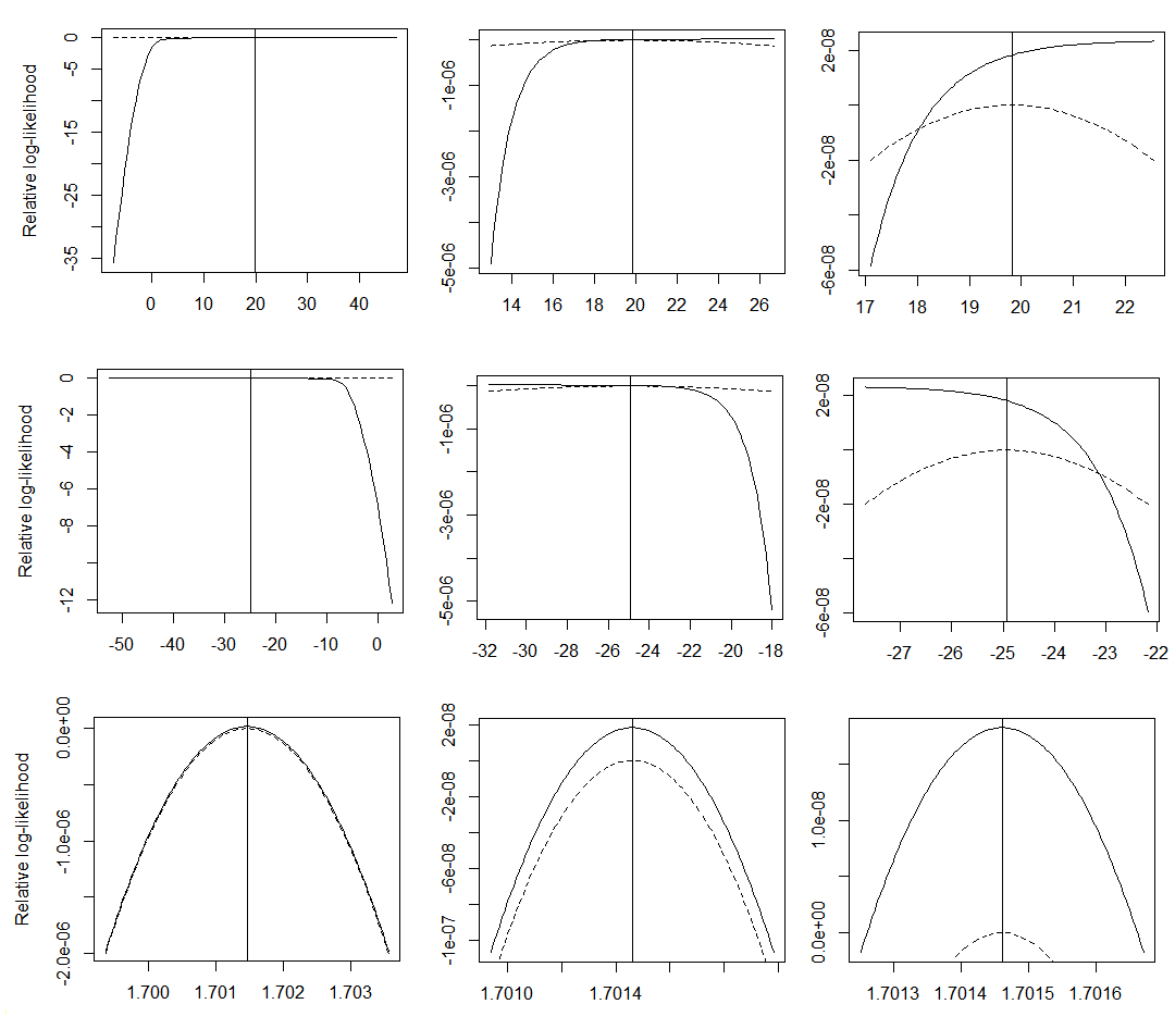
The following plot shows the log-likelihood function with respect to a positive infinite coefficient, a negative infinite coefficient, and a regular coefficient by row at gradually finer scales by column, respectively. The dotted curve, almost a straight line in a large scale corresponding to an infinite estimate, is the quadrative approximation that the Wald test makes at the point where the vertical line, representing the maximum-likelihood estimate, intersects the log-likelihood function. It is the strong asymmetry in the log-likelihood function that undermines the performance of Wald tests.

To compare Wald, score, and likelihood-ratio statistics in practice, I enhance the toy data described by Hauck and Donner (1977) by varying the sample size of the reference group.

Data_Temp <- list()
for(k in c(4, 8, 16, 32, 64, 100, 500, 1000, 10000)) {
  Data_Temp[[1]] <- data.frame(x = c(rep(0, k), rep(1, 100)))
  Data_Temp[[2]] <- data.frame(j = NA, b = NA, wald = NA, score = NA, lrt = NA)
  for(j in 1:99) {
    Data_Temp[[1]] <- Data_Temp[[1]] %>%
      mutate(y = c(
        rep(1, k * 0.25), rep(0, k * 0.75), 
        rep(1, j), rep(0, 100 - j)))
    Model_Temp <- glm(y ~ x, data = Data_Temp[[1]], family = poisson())
    Data_Temp[[2]][j, "j"] <- j
    Data_Temp[[2]][j, "b"] <- Model_Temp$coefficients[2]
    Data_Temp[[2]][j, "wald"] <- (summary(Model_Temp)$coefficients[2, 3])^2
    Data_Temp[[2]][j, "score"] <- drop1(Model_Temp, test = "Rao")[2, 4]
    Data_Temp[[2]][j, "lrt"] <- drop1(Model_Temp, test = "LRT")[2, 4]
  }
  Data_Temp[[3]] <- if(length(Data_Temp) < 3) 
    Data_Temp[[2]] %>% bind_cols(n0 = as.integer(k)) 
  else Data_Temp[[3]] %>% bind_rows(
    Data_Temp[[2]] %>% bind_cols(n0 = as.integer(k)))
}

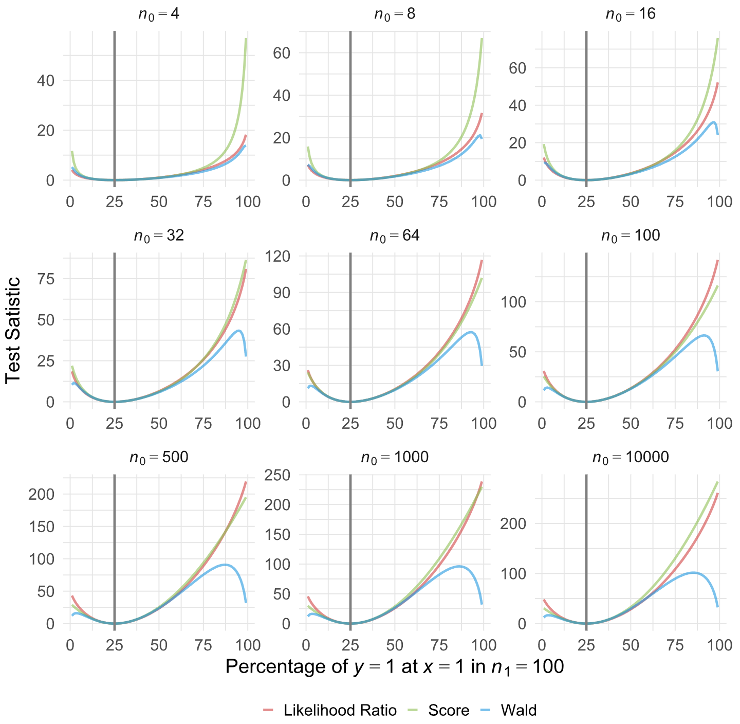
Using the three test methods to test the significance of the single binary predictor in a series of binary logit regression models give the following plot. The boundary issue with Wald tests happens on both sides of extremities, representing odds in the treatment group at zero and infinity, respectively. Also clearly shown is that increasing the total sample size does not resolve the abnormal Wald behavior. Wald tests usually but not always report p values larger than those from likelihood-ratio tests. When the sample sizes across x levels are balanced, likelihood-ratio tests are most powerful for giving the largest statistic. When the sample sizes are imbalanced, however, score tests can give the largest statistic in some parameter regions.

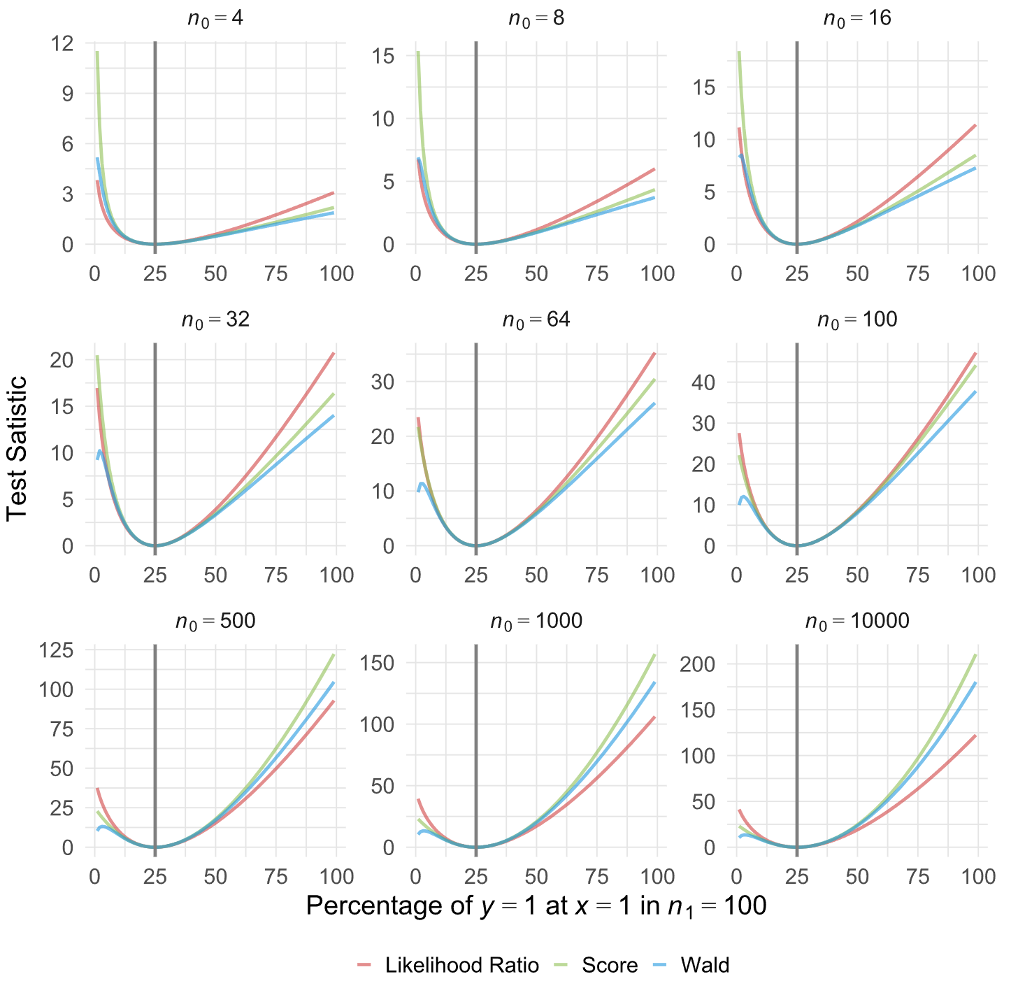
Fitting Poisson regression models to the same data result in the following plot. The boundary issue with Wald tests happens on only one side of extremities, representing incident rates (proportion of y = 1 when x = 1) at zero in the treatment group of a sample size n1 = 100. For lower incident rates in the treatment group than in the reference group (0.25), β < 0, score tests give the largest statistics for small sample size in the reference group (n0 <= 64), whereas likelihood ratio give the largest statistic in larger reference groups. The Wald-test statistic can be either smaller or larger than likelihood-ratio result. When β > 0, however, likelihood ratio give the largest statistic in smaller reference groups and the smallest statistic in larger reference groups. Your estimation roughly mimics the case in the middle panel, where n0 = 64 and y = 1 in 25% of the observations while n1 = 100 and y = 1 in none of the observations.

In all cases of both logit and Poisson models, score tests appear to always give larger statistics than Wald tests. Likelihood ratio tests can give either smaller or larger than Wald and score tests, depending on the coefficient sign and sample balance.

• Buse, A. (1982). The likelihood ratio, Wald, and Lagrange multiplier tests: An expository note. The American Statistician, 36(3), 153–157. https://doi.org/10.2307/2683166

• Christensen, R. H. B. (2022). Cumulative link models for ordinal regression with the R package ordinal. https://cran.r-project.org/web/packages/ordinal/vignettes/clm_article.pdf

• Freedman, D. A. (2007). How can the score test be inconsistent? The American Statistician, 61(4), 291–295. https://doi.org/10.1198/000313007X243061

• Freeman, E., Keele, L., Park, D., Salzman, J., & Weickert, B. (2015). The plateau problem in the heteroskedastic probit model (arXiv:1508.03262). arXiv. https://doi.org/10.48550/arXiv.1508.03262

• Greene, W. H., & Hensher, D. A. (2010). Modeling ordered choices: A primer. Cambridge University Press.

• Hauck, W. W., Jr., & Donner, A. (1977). Wald’s test as applied to hypotheses in logit analysis. Journal of the American Statistical Association, 72(360), 851–853. https://doi.org/10.1080/01621459.1977.10479969

• Rao, C. R. (2005). Score test: Historical review and recent developments. In N. Balakrishnan, H. N. Nagaraja, & N. Kannan (Eds.), Advances in Ranking and Selection, Multiple Comparisons, and Reliability: Methodology and Applications (pp. 3–20). Birkhäuser. https://doi.org/10.1007/0-8176-4422-9_1

• Yee, T. W. (2021). On the Hauck–Donner effect in Wald tests: Detection, tipping points, and parameter space characterization. Journal of the American Statistical Association, 0(0), 1–12. https://doi.org/10.1080/01621459.2021.1886936

Answer 4

The two tests are asymptotically equivalent. Of course, their performance (size and power) in finite samples can differ. The best you can do to understand the difference is to run a Monte Carlo study for a setting similar to yours.

Answer 5

Just a few minor comments. It's bad style using $ in an R formula; use the 'data' argument instead. Also, care is needed when hypothesis testing a null value that lies on the boundary, for example, the ZIP. I think Self and Liang have a JASA paper on that. Having one observation per group is definitely not conducive to results based on asymptotics. Here, that's one coefficient per observation, so it violates the usual conditions required for asymptotic results to kick in.

Two more thoughts: hypothesis testing must involve nested models. And the score statistic sometimes has its information computed at the MLE. If so, then it may become inaccurate near the boundary due to the same reason the Wald statistic exihibits the HDE in that region of the parameter space.

BTW, can you please make available the code for producing the graphics? Thanks.

Answer 6

Quoting @jsakaluk quoting Agresti:

When the sample size is small to moderate, the Wald test is the least reliable of the three tests. We should not trust it for such a small n as in this example (n = 10).

I wanted to get a sense for Wald's test reliability. Here's a simple simulation of 10000 tests of two groups with mean 10 and 12, sd = 1, N = 5 per group:

library(lmtest)
library(aod)

n <- 5
x <- rep(c('A', 'B'), each=n)

wtp <- rep(NA, 10000) 
lrtp <- rep(NA, length(wtp))
for (i in 1:length(wtp)) {
    set.seed(i)
    y <- c(rnorm(n=n, mean=10), rnorm(n=n, mean=12))
    fit <- lm(y ~ x)

    # Wald test
    wt <- wald.test(Sigma=vcov(fit), b=coef(fit), Terms=2)$result$chi2
    p <- wt[names(wt) == 'P']
    wtp[i] <- p

    # LRT
    fit0 <- lm(y ~ 1)
    tt <- lrtest(fit0, fit)
    lrtp[i] <- tt[['Pr(>Chisq)']][2]
}

Plot the resulting pvalues from the two methods:

plot(-log10(wtp), -log10(lrtp), pch=19, cex=0.5, xlab='Wald test', ylab='LRT', main=sprintf('-log10(pvalue) for %d tests', length(wtp)))
grid()
abline(a=0, b=1, col='blue')

It seems to me that with such small n (5), Wald gives unrealistically small p-values too often. Number of tests with p < 1e-6:

sum(wtp < 10e-6)
2248

sum(lrtp < 10e-6)
285

Tests with p > 0.01:

sum(wtp > 0.01)
2832

sum(lrtp > 0.01)
3312