11
$\begingroup$

Let's say that I generate the probability of an outcome based on a certain factor and plot the curve of that outcome. Is there any way to extract the equation for that curve from R?

> mod = glm(winner~our_bid, data=mydat, family=binomial(link="logit"))
> summary(mod)

Call:
glm(formula = winner ~ our_bid, family = binomial(link = "logit"), 
    data = mydat)

Deviance Residuals: 
    Min       1Q   Median       3Q      Max  
-0.7443  -0.6083  -0.5329  -0.4702   2.3518  

Coefficients:
              Estimate Std. Error z value Pr(>|z|)    
(Intercept) -9.781e-01  2.836e-02  -34.49   <2e-16 ***
our_bid     -2.050e-03  7.576e-05  -27.07   <2e-16 ***
---
Signif. codes:  0 ‘***’ 0.001 ‘**’ 0.01 ‘*’ 0.05 ‘.’ 0.1 ‘ ’ 1 

(Dispersion parameter for binomial family taken to be 1)

    Null deviance: 42850  on 49971  degrees of freedom
Residual deviance: 42094  on 49970  degrees of freedom
AIC: 42098

Number of Fisher Scoring iterations: 4

> all.x <- expand.grid(winner=unique(winner), our_bid=unique(our_bid))
> all.x
> won = subset(all.x, winner == 1)
> y.hat.new <- predict(mod, newdata=won, type="response")
> options(max.print=5000000)
> y.hat.new
> plot(our_bid<-000:1000, predict(mod, newdata=data.frame(our_bid<-c(000:1000)),
       type="response"))
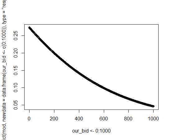
enter image description here

How can I go from this probability curve to an equation in R? I was hoping for something like:

Probability = -0.08*bid3 + 0.0364*bid2 - 0.0281*bid + 4E-14
$\endgroup$
1
  • 2
    $\begingroup$ Unlike the example in your code, which has one independent variable (bid) and therefore plots as a curve in a (bid, probability) plane, the example in your edit at the end would not plot as a curve: it would be a three -dimensional hypersurface plotted in four dimensions (bid, bid2, bid3, probability). $\endgroup$
    – whuber
    Commented Jan 9, 2012 at 18:51

1 Answer 1

16
$\begingroup$

This generalized linear model supposes the outcome associated with an independent value of $x$ has a binomial distribution whose log odds ("logit") vary linearly with $x$. The output provides the coefficients of that linear relation; namely, the intercept is estimated as -0.9781 and the slope ("our_bid") as -0.002050. You can see them in the Estimate column:

              Estimate Std. Error z value Pr(>|z|)    
(Intercept) -9.781e-01  2.836e-02  -34.49   <2e-16 ***
our_bid     -2.050e-03  7.576e-05  -27.07   <2e-16 ***

The probability, which you wish to plot, is related to the log odds by

$$\text{probability} = \frac{1}{1 + \exp(-\text{log odds})}.$$

R calls this the "inverse logit" function, inv.logit.

Putting these together gives the equation

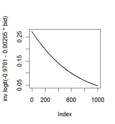
$$\text{probability} = \frac{1}{1 + \exp\left(-[-0.9781 - 0.00205 x]\right)}.$$

An R command to plot it would be

plot(inv.logit(-0.9781 - 0.00205*(0:1000)))

Plot output

In general, you should extract these coefficients with the coefficients command rather than transcribing them (as I did here, because I do not have access to your data).

$\endgroup$
1
  • 3
    $\begingroup$ (+1) Of note, the Hmisc::latex function makes it easy to print the above as $\LaTeX$, e.g. latex(fit.1) may yield this output (using sample code here). $\endgroup$
    – chl
    Commented Jan 9, 2012 at 19:44

Your Answer

By clicking “Post Your Answer”, you agree to our terms of service and acknowledge you have read our privacy policy.

Not the answer you're looking for? Browse other questions tagged or ask your own question.