Is correlation between a parameter and the log posterior inherently problematic?

Question

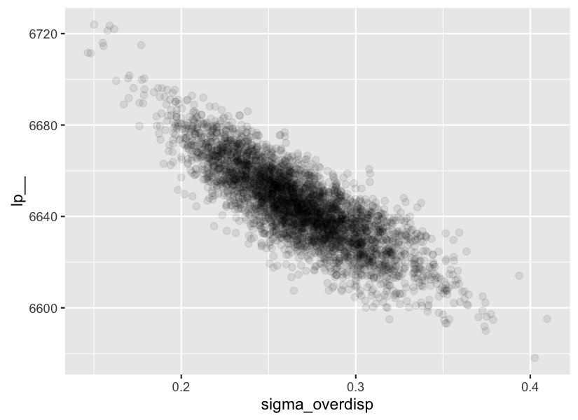
In fitting quasi-Poisson models using RStan, I often see a negative correlation between the variance of the overdispersion term and the overall log posterior (lp__). Other diagnostics such as Rhat, effective sample size, and trace plots look good. Is a correlation between a model parameter and lp__ inherently problematic (i.e. indicate a lack of convergence or other problem with the model)?

Example:

Quasi-Poisson RNG function to generate overdispersed-Poisson counts (with variance = mean * theta):

rqpois <- function(n, mu, theta) {
  rnbinom(n = n, mu = mu, size = mu/(theta-1))
}

Generate counts y as log-link function of continuous variable x:

set.seed(4536)
N <- 200
x <- runif(N, 0, 10)
alpha <- 1
beta <- 0.3
y_pred <- exp(alpha + beta * x)
y <- rqpois(n = N, mu = y_pred, theta = 2)

Stan model:

qpois_stan <- "
  data {
    int<lower=0> N;
    real<lower=0> x[N];
    int<lower=0> y[N];
  }

  parameters {
    real alpha;
    real beta;
    vector[N] overdisp;
    real<lower=0> sigma_overdisp;
  }

  transformed parameters {
    vector[N] mu;

    for(i in 1:N) {
      mu[i] <- alpha + beta * x[i] + overdisp[i];
    }
  }

  model {
    alpha ~ normal(0, 10);
    beta ~ normal(0, 10);
    overdisp ~ normal(0, sigma_overdisp);
    sigma_overdisp ~ cauchy(0, 10);

    y ~ poisson_log(mu);
  }"

Fit model using rstan:

mod <- stan(
  model_code = qpois_stan,
  data = list(N = N, x = x, y = y),
  warmup = 2000,
  iter = 4000,
  chains = 2
)

Negative correlation between lp__ and sigma_overdisp:

Answer 1

That's OK. You expect a strong relationship between the parameters and the log density. Sometimes it's U-shaped with a clear maximum marginal likelihood that is within the sampled posterior and sometimes like what you show. The Bayesian posterior won't necessarily include the maximum likelihood estimate or anything near it in the posterior. Instead, it gives you the typical set, which is the kind of draws you'd expect if you could draw from the posterior at random. This is why you can get posteriors in cases like hierarchical models where there is no maximum likelihood estimate (only marginal maximum likelihood estimates as produced by packages like lme4).

You should be able to see this if you plot the log density vs. sigma_overdisp with the other parameters fixed to some reasonable value.