3
$\begingroup$

I am not sure in the terminology, so I will simply try to explain the situation that I would like to model as I see it. Suppose there is a set of random variables. The variables are correlated in such a way that they deviate from their expected values into the same direction all together. By this I mean that they can be either all together larger then their expectation or all together lower. Is it possible to model such a dependency with a multivariate normal random variable $\mathbf{X} \sim \mathcal{N}(\mathbf{\mu}, \mathbf{\Sigma})$, assuming the knowledge about the marginal distributions of the components $\mathbf{X}_i \sim \mathcal{N}(\mu_i, \sigma^2_i)$? How to construct $\mathbf{\Sigma}$ is this situation? Thank you.

Best wishes, Ivan

$\endgroup$
18
  • 1
    $\begingroup$ If you require that there be no possibility of deviations from this correlated behavior, then these variables cannot be multivariate normal unless they all are linear combinations of a constant and one (univariate) normal. But perhaps your restriction is not as severe as this? $\endgroup$
    – whuber
    Commented Feb 17, 2012 at 15:10
  • $\begingroup$ Unless I misunderstand the question, can't you just fill $\mathbf{\Sigma}$ in with the covariances from your dataset? $\endgroup$
    – rm999
    Commented Feb 17, 2012 at 15:14
  • $\begingroup$ Thank you for the replies. The point is that I am trying to build a model of a quite complicated system and, in order to be able to at least start from something, I can make some assumptions that later, I hope, I will be able to get rid of or relax. Since multivariate r.v.'s are quite comfortable to deal with (and the nature is supposed to be fair), I have decided to start from them, but the correlation mentioned earlier is a must, it should be in the model from the very beginning. $\endgroup$
    – Ivan
    Commented Feb 17, 2012 at 15:36
  • 1
    $\begingroup$ @whuber, I also though about this possibility of having just one normal r.v. $\xi$, the rest are just linear transformations of it like $\mathbf{X}_i = a_i \xi + b_i$. May be I should start from this simple scenario. $\endgroup$
    – Ivan
    Commented Feb 17, 2012 at 15:39
  • $\begingroup$ @rm999, probably, you are also right. If one has a bunch of data, based on which s/he estimates $\mu_i$ and $\sigma^2_i$, s/he can also try to estimate the covariance matrix. $\endgroup$
    – Ivan
    Commented Feb 17, 2012 at 15:42

1 Answer 1

3
$\begingroup$

Consider this very simple snippet:

    m1 <- 0
    m2 <- 0
    cov <- 0.8
    x1 <- rnorm(100, mean=m1)
    x2 <- cov*x1 + rnorm(100,mean=m2-cov*m1,sd=sqrt(1-cov*cov))
    plot(x1,x2)
    x2a <- x2*sign(x1-m1)*sign(x2-m2)
    plot(x1,x2a)

It folds the distribution of x2 around its mean, aligning its deviations from the mean to those of x1 from its mean. Of course the resulting distribution cannot be characterized as a multivariate normal, although each margin is normal:

    plot( density(x1), ylim=c(0,0.5) )
    hist( x1, add=T, prob=T )

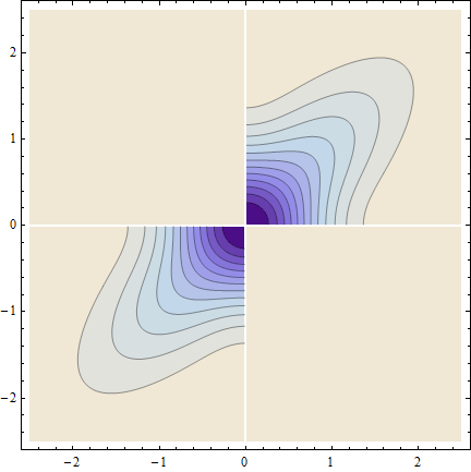
Contour

Contours of the density of (x1, x2a): the probability that would ordinarily be associated with values in quadrants II or IV has been symmetrically displaced into quadrants I and III, leaving the marginal distributions undisturbed.

This is a classic (counter)example of a distribution that has normal margins, yet is not a multivariate normal; frankly, I don't know how to build any other ones.

The transformation increases the correlation somewhat:

    > cor(x1,x2)
    [1] 0.7999774
    > cor(x1,x2a)
    [1] 0.8575814

You would've seen a much stronger effect with lower cov, of course: you can start with cov=0 and still get the correlation of the resulting variables above 0.6.

$\endgroup$
5
  • 2
    $\begingroup$ When starting with a bivariate normal distribution of correlation $\rho\ge 0$, this procedure produces a bivariate distribution of correlation $\frac{2}{\pi}(\sqrt{1-\rho^2}+\rho \arcsin(\rho))$, which ranges from $2/\pi\approx 0.637$ up to $1$. $\endgroup$
    – whuber
    Commented Feb 17, 2012 at 18:57
  • $\begingroup$ @whuber, do you have a reference? Not that I am not ready to take your word for it, but to have a complete response. It would also be great if you could post the contour plot code if you have it at your fingertips. $\endgroup$
    – StasK
    Commented Feb 17, 2012 at 20:04
  • 1
    $\begingroup$ The results in the comment are just a calculation. (And you shouldn't take my word for it: I make mistakes. But at least the formula agrees with your results! It gives 0.854 for $\rho=0.8$.) For the plot, here's Mathematica code: $\endgroup$
    – whuber
    Commented Feb 17, 2012 at 20:18
  • $\begingroup$ $\text{With}[\{\mu=0,\nu=0, \sigma=1, \tau=1, \rho=\frac{4}{5}\},$ $g[\text{x_},\text{y_}] \text{:=}\text{With}[\{f = \text{BinormalDistribution}[\{\mu , \nu \},\{\sigma , \tau \},\rho ]\},$ $\quad\text{Piecewise}[\{\{\text{PDF}[f, \{x,y\}] + \text{PDF}[f, \{2\mu -x,y\}], (x-\mu )(y-\nu )\geq 0\}\}, 0]];$ $\text{ContourPlot}[g[x,y], \{x,\mu -2.5\sigma ,\mu +2.5\sigma \}, \{y,\nu -2.5\tau ,\nu +2.5\tau \},$ $\quad\text{PlotRange}\to \{\text{Full}, \text{Full}, \text{Full}\}, \text{Contours}\to 12,$ $\text{PlotPoints}\to 100, \text{AspectRatio}\to \tau /\sigma ]]$ $\endgroup$
    – whuber
    Commented Feb 17, 2012 at 20:18
  • 2
    $\begingroup$ Related to @whuber's calculation: Recent MO question and answer. $\endgroup$
    – cardinal
    Commented Feb 17, 2012 at 22:05

Your Answer

By clicking “Post Your Answer”, you agree to our terms of service and acknowledge you have read our privacy policy.

Not the answer you're looking for? Browse other questions tagged or ask your own question.