heteroscedasticity, residual vs. independent X variables in a multiple regression

Question

My Y variable varies between 0 and 1 with increments of 0.067. I have a lot of zeros in my data. My questions are:

1. Is the residual vs. fitted plot below OK. Or as suggested in this link: Heteroscedasticity in residuals vs. fitted plot and this link: How should I interpret this residual plot? is there a floor effect? Do I need to consider a different type of model, perhaps a logistic model?

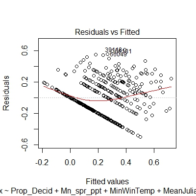
2. Neter et al (1989) in p247 advises 'residuals should be plotted against each independent variables.' If moderate heteroscedasticity is not an issue in residual vs. fitted plot, do I have to check for heteroscedasticity in residual vs. each individual X variable? Asking the same question differently, if my residual vs. fitted plot is fine in model Y ~ X1 + X2 + X3 + X4 + X5 (not the one in the image above), but residual vs. X4 shows heteroscedasticity, what do I do?

Answer 1

You have count data - use a model appropriate for this: Based on your description of the data, and your residual plot, I suggest that your response variable is a proportion value based on a fixed denominator, which means that it is based on an underlying set of count data (i.e., positive integers up to a fixed known maximum value). That is why you get lines of values in your residual plot when you use OLS estimation. In such cases, the error term in them model is not normally distributed, and you will probably get a better fit from a model designed for count data (e.g., a binomial GLM).

Answer 2

I would use a different type of model. The lm() function in R fits a model with normally distributed errors. The normal distribution is unbounded, meaning it can take any value between -Inf and Inf. In contrast, your response is bounded. Heteroscedasticity (variance changing with the fitted response value) is an issue for models with normal errors as they assume a constant variance.

1. You should fit a model with binomial errors. You can do this with:

glm(l Y ~ X1 + X2 + X3 + X4 + X5, family = binomial, data = df)

GLMs with binomial errors cannot be checked by eye easily and you should not expect them to look like a white-noise residual plot (like the ones we hope to see with lms). Unfortunately, there is no simple way to check the assumptions of a binomial glm.

2. In the case of multiple linear regression you do not need to plot the residuals by each variable. The residual v.s. fitted plot is typically enough.