How to describe variation on multiple levels?

Question

This is continuation for a series of questions (1, 2). I have a data set from an experiment with 2x2 design. A replicate consists of 20-50 normally distributed replicate measurements. Each treatment combination has 3 of these replicates. Measured average response for each replicate seems not to be normally distributed.

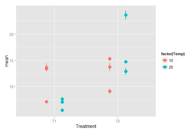
Figure 1. Example of the problem. Error bars show standard error of mean.

Since this is an experiment and I am supposed to talk about an effect of a treatment, I would like to combine the variation within measurements (error bars) and between replicates (dots in the figure) into one number / treatment combination and use the error bars with one mean value to show the overall effect of a treatment (a dot instead of three). Ideally I would like to use confidence intervals of some sort (asked here). I have understood that since this is an unbalanced nested design, I should use mixed models or a simple 2-way ANOVA for mean values, but how to compress the variation on two levels into one figure?

Would the delta method be something for me?

R code with an example of the data:

library(ggplot2)

x1 <- c(rnorm(50, 14,3),rnorm(35, 7,1),rnorm(40, 15,9))
x2 <- c(rnorm(43, 6,3),rnorm(32, 7,1),rnorm(40, 8,4))
x3 <- c(rnorm(50, 15,5), rnorm(50, 10,7), rnorm(50, 13,9))
x4 <- c(rnorm(26, 14,2), rnorm(43, 25,10), rnorm(45, 15,9))

dx1 <- data.frame(Treatment = rep("T1", length(x1)), Temp = rep(10, length(x1)), Rep = rep(c(1,2,3), times = c(50,35,40)), Meas = x1)
dx2 <- data.frame(Treatment = rep("T1", length(x2)), Temp = rep(20, length(x2)), Rep = rep(c(4,5,6), times = c(43,32,40)), Meas = x2)
dx3 <- data.frame(Treatment = rep("T2", length(x3)), Temp = rep(10, length(x3)), Rep = rep(c(7,8,9), times = c(50,50,50)), Meas = x3)
dx4 <- data.frame(Treatment = rep("T2", length(x4)), Temp = rep(20, length(x4)), Rep = rep(c(10,11,12), times = c(26,43,45)), Meas = x4)

# Entire data set

dat <- rbind(dx1,dx2,dx3,dx4)

# Plot overview

w <- ggplot(dat, aes(x = factor(Rep), y = Meas))
w + geom_boxplot(aes(fill = factor(Temp)))

# Averages (with se)

aveg <- aggregate(Meas ~ Treatment + Temp + Rep, data = dat, FUN = mean)
se <- function(x) sd(x)/sqrt(length(x))
SE <- aggregate(Meas ~ Treatment + Temp + Rep, data = dat, FUN = se)

dat2 <- merge(aveg, SE, by = c("Treatment", "Temp", "Rep"), sort = F)

colnames(dat2)[colnames(dat2) %in% grep("\\.x", colnames(dat2), value = T)] <- "mean"
colnames(dat2)[colnames(dat2) %in% grep("\\.y", colnames(dat2), value = T)] <- "se"

# Plot entire data set

p <- ggplot(dat2, aes(x = Treatment, y = mean, ymax = mean + se/2, 
ymin = mean - se/2))

p + geom_pointrange(aes(color = factor(Temp)), 
position=position_dodge(width=0.50), size = 1)

Answer 1

For simplicity, first consider only one group. Your data can be modeled as $$Y_{ij} = \mu + \delta_i + \epsilon_{ij},$$ where $\delta_i \sim N(0, \tau^2), i=1,\ldots,k$ is the random day effect, and $\epsilon_{ij}\sim N(0, \sigma^2), j=1,\ldots, n_i$ is the random within-day replicate effect. Then you can obtain an unbiased estimate of the group average $$\hat\mu = \frac 1k \sum_{j=1}^j \bar{Y}_{i.} \sim N(\mu, \frac{\tau^2}{k} + \frac 1k \sum_{i=1}^k \frac{\sigma^2}{n_i}).$$ It is fairly simple to obtain estimates of the variance term with $\tau^2$ being the variance of the day means, and $\sigma^2$ the pooled within-day variance.

Start edit

The variance term in this formula gives you the square of the standard error for your plot. The point to show would be the mean of the within-day means. If you don't want to assume that the within-day variability is constant, just replace $\sigma$ with $\sigma_i$ - the within-day standard deviation on day 1, so the summation would be $\sum_iSE_i^2$, where $SE_i$ is the standard error of the within-day mean.

End edit

If for a moment you assume $n_i=n$, then the variance is $\frac{\tau^2}{k} + \frac{\sigma^2}{n}$. In your application the key observation is that $n >> k$, so the first term will dominate. In essence, you can ignore the within-day replicates, and just use them as an expensive way to obtain one (day-specific) observation.

I have run a "correct" mixed ANOVA analysis and a simple ANOVA on group means, and they give essentially the same result:

library(lme4)
m1 <- lmer(Meas ~ Treatment*Temp + (1|Rep), data=dat)
m1

Output:

Linear mixed model fit by REML 
Formula: Meas ~ Treatment * Temp + (1 | Rep) 
   Data: dat 
  AIC  BIC logLik deviance REMLdev
 3351 3376  -1669     3343    3339
Random effects:
 Groups   Name        Variance Std.Dev.
 Rep      (Intercept) 15.414   3.9260  
 Residual             42.000   6.4808  
Number of obs: 504, groups: Rep, 12

Fixed effects:
                 Estimate Std. Error t value
(Intercept)       16.1579     5.2369   3.085
TreatmentT2       -9.3838     7.3903  -1.270
Temp              -0.4723     0.3315  -1.425
TreatmentT2:Temp   1.0377     0.4683   2.216

And

m2 <- lm(mean ~ Treatment*Temp, data=dat2)
summary(m2)

with output

Coefficients:
                 Estimate Std. Error t value Pr(>|t|)  
(Intercept)       16.1037     5.2451   3.070   0.0153 *
TreatmentT2       -9.2846     7.4177  -1.252   0.2460  
Temp              -0.4694     0.3317  -1.415   0.1948  
TreatmentT2:Temp   1.0302     0.4691   2.196   0.0594 .
---
Signif. codes:  0 ‘***’ 0.001 ‘**’ 0.01 ‘*’ 0.05 ‘.’ 0.1 ‘ ’ 1 

Residual standard error: 4.063 on 8 degrees of freedom
Multiple R-squared: 0.5955,     Adjusted R-squared: 0.4438 
F-statistic: 3.926 on 3 and 8 DF,  p-value: 0.05412