0
$\begingroup$

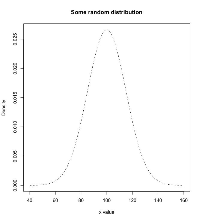
I have the following randomly generated distribution:

mean=100; sd=15
x <- seq(-4,4,length=100)*sd + mean
hx <- dnorm(x,mean,sd)

plot(x, hx, type="l", lty=2, xlab="x value",
     ylab="Density", main="Some random distribution")

enter image description here

And a "non-random" value

x <- seq(-4,4,length=100)*10 + mean
ux <- dunif(x = x, min=10, max=100)
non_random_value <- ux[1]
non_random_value
# [1] 0.01111111

I'd like to have the statistic that show non_random_value is significant and doesn't come up by chance with respect to hx.

What is the reasonable statistics to check that?

$\endgroup$
3
  • 2
    $\begingroup$ Two common approaches would be p-value (based on just the normal PDF) and bayes-factors (comparing the normal vs. uniform PDFs). $\endgroup$
    – GeoMatt22
    Commented Apr 29, 2017 at 3:08
  • 2
    $\begingroup$ @GeoMatt22: Can you give specific example, e.g. R code? I'm here comparing one value versus one distribution. $\endgroup$
    – neversaint
    Commented Apr 29, 2017 at 9:03
  • 1
    $\begingroup$ Literally any number allowed by a distribution can "come up by chance." This, therefore, is not a testable statement. What is the problem you really face? $\endgroup$
    – whuber
    Commented May 5, 2017 at 14:08

2 Answers 2

4
+25
$\begingroup$

How do you define "by chance"? I ask because the answer to the question asked like this is very simple and very unlikely to give any meaningful results.

If you have random variable $X$ that follows a distribution described by a cumulative distribution function $F$, then to answer your question you need to simply decide about some arbitrary probability cut-off $\alpha$ and then check if

$$ \Pr(X > x) = 1-F(x) < \alpha $$

or

$$ \Pr(X < x) = F(x) > 1-\alpha $$

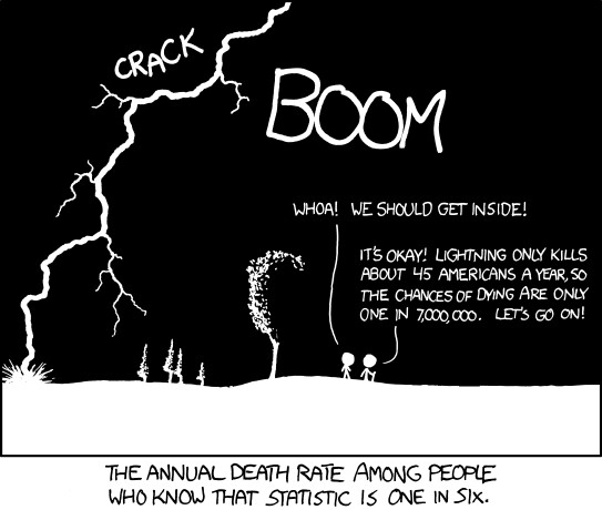
depending on your hypothesis. Where $x$ is your value of interest. However doing so will led you to meaningless results, e.g. that any human cannot be hit by a thunderbolt "by chance" if it happens with probability less then $\alpha$...

xkcd comic

(source: xkcd.com)

$\endgroup$
1
$\begingroup$

The easiest way is to convert your distribution to a density, and calculate a one tailed p-value by integrating.

#Original OPs code
mean=100; sd=15
x <- seq(-4,4,length=100)*sd + mean
hx <- dnorm(x,mean,sd)
plot(x, hx, type="l", lty=2, xlab="x value",
ylab="Density", main="Some random distribution")
x <- seq(-4,4,length=100)*10 + mean
ux <- dunif(x = x, min=10, max=100)
non_random_value <- ux[1]
non_random_value
# [1] 0.01111111

If your hypothesis is that non_random_value is larger than you would randomly obtain from the distribution than by chance, than:

library("sfsmisc")
hx_den=density(hx)
pvalue=integrate.xy(hx_den$x,hx_den$y,non_random_value,max(hx_den$x))
pvalue
#[1] 0.3319186 # not statistically significant

If your hypothesis is that non_random_value is smaller than you would obtain from the distriubtion than by chance, than:

library("sfsmisc")
pvalue=integrate.xy(hx_den$x,hx_den$y,min(hx_den$x),non_random_value)
pvalue
#0.6685339 # not statistically significant either
$\endgroup$
6
  • 5
    $\begingroup$ The unmotivated appearance of "one-tailed" in this answer belies a rather large set of implied suppositions that you need to make explicit. How do you view this as a hypothesis test? What is the null hypothesis? What is the alternative hypothesis? It's not hard to find examples that make these calculations look rather silly. For instance, consider an equal mixture of uniform distributions supported on $(-2,-1)$ and $(1,2)$. Your calculation gives a "p-value" of $1/2$ for the impossible, zero-chance result of $0$! Clearly, then, you have to make assumptions that rule out such examples. $\endgroup$
    – whuber
    Commented May 5, 2017 at 14:07
  • 2
    $\begingroup$ @whuber the pvalue here is simply the probability of generating the point or a point more extreme on one tail or another given the distribution. The alternative is that the point is not from the distribution below or above the extremes. Your example is contrived (while technically correct), and my "implied suppositions" are consistent with the OP's example, where the non random value has a non-zero probability of occurring in the original distribution. $\endgroup$
    – Josh
    Commented May 5, 2017 at 14:29
  • 3
    $\begingroup$ It's a little contrived, but only to make the point clear: the situation is quite realistic. Almost any bimodal distribution would cause the same problem. I am suggesting that the difficulty with your answer is both conceptual and fundamental. In the absence of a clearly articulated and relevant null and alternative hypothesis, your calculation has no justification and very well could lead to completely wrong decisions. $\endgroup$
    – whuber
    Commented May 5, 2017 at 15:19
  • 2
    $\begingroup$ @whuber, I disagree. If OP were to clarify a specific alternative hypothesis (e.g. another distribution), that would be great. However, in many cases, no practical alternative exists, and all we have is the data in front of us. Asking whether the model explains the data is useful for deciding other models to explore. If I told you that I had a model with a normal distribution with mean=0 and sd=1, and I had a point=1,000,000, are you really willing to say that I really know nothing about whether the model is truly correct? $\endgroup$
    – Josh
    Commented May 5, 2017 at 15:42
  • $\begingroup$ @user3923510 So according to your method, we cannot accept that non_random_value is significant and doesn't come up by chance with respect to hx? $\endgroup$
    – neversaint
    Commented May 6, 2017 at 0:26

Your Answer

By clicking “Post Your Answer”, you agree to our terms of service and acknowledge you have read our privacy policy.

Not the answer you're looking for? Browse other questions tagged or ask your own question.