14
$\begingroup$

As I'm sure everyone here knows already, the PDF of the Beta distribution $X \sim B(a,b)$ is given by

$f(x) = \frac{1}{B(a,b)}x^{a-1}(1-x)^{b-1}$

I've been hunting all over the place for an explanation of the origins of this formula, but I can't find it. Every article I've found on the Beta distribution seems to give this formula, illustrate a few of its shapes, then go straight on to discussing its moments and on from there.

I don't like using mathematical formulae I can't derive and explain. For other distributions (e.g. the gamma or the binomial) there's a clear derivation I can learn and use. But I can't find anything like that for the Beta distribution.

So my question is: what are the origins of this formula? How can it be derived from first principles in whatever context it was originally developed?

[To clarify, I'm not asking about how to use the Beta distribution in Bayesian statistics, or what it means intuitively in practice (I've read the baseball example). I just want to know how to derive the PDF. There was a previous question that asked something similar, but it was marked (I think incorrectly) as a duplicate of another question that did not address the issue, so I haven't been able to find any help on here so far.]

EDIT 2017-05-06: Thanks everyone for the questions. I think a good explanation of what I want comes from one of the answers I got when I asked this of some of my course instructors:

"I guess people could derive the normal density as a limit of a sum of n things divided by sqrt(n), and you can derive the poisson density from the idea of events occurring at a constant rate. Similarly, in order to derive the beta density, you would have to have some kind of idea of what makes something a beta distribution independantly from, and logically prior to, the density."

So the "ab initio" idea in the comments is probably closest to what I'm looking for. I am not a mathematician, but I feel most comfortable using mathematics that I can derive. If the origins are too advanced for me to handle, so be it, but if not I would like to understand them.

$\endgroup$
10
  • 5
    $\begingroup$ Derived from what? If the binomial-conjugate-prior approach is not acceptable, several alternatives are here (e.g. order statistics of a uniform random variable, proportions of Gamma variables). $\endgroup$
    – GeoMatt22
    Commented May 4, 2017 at 20:33
  • 3
    $\begingroup$ Note: the whole history of the Beta distribution is provided in the unbelievable Wikipedia page on this distribution, which contains about every possible detail! $\endgroup$
    – Xi'an
    Commented May 4, 2017 at 21:00
  • 1
    $\begingroup$ The previous question was marked as a duplicate of the other after the OP clarified what they were after in a comment. whuber asked the same question there as @Geomatt22 does here: "A derivation means a logical connection from something assumed to something to be established. What do you want to assume?" $\endgroup$
    – Scortchi
    Commented May 4, 2017 at 21:06
  • 2
    $\begingroup$ @Aksakal but then the question is too broad -- it may be derived an all manner of ways; if you're right, I'll close it as too broad until the question is narrowed down enough to be something other than a grab bag of possible answers $\endgroup$
    – Glen_b
    Commented May 5, 2017 at 3:15
  • 3
    $\begingroup$ Some brief discussion of a little historical context is here (at least in terms of its relationship to the incomplete beta function). It has connections to the gamma distribution, and many, many other distributions besides and arises quite reasonably in a number of different ways; as Xi'an points out it's also got historical origins in the Pearson system. What kind of answer are you seeking here? What's given/what must be derived? $\endgroup$
    – Glen_b
    Commented May 5, 2017 at 3:16

3 Answers 3

8
$\begingroup$

As a former physicist I can see how it could have been derived. This is how physicists proceed:

when they encounter a finite integral of a positive function, such as beta function: $$B(x,y) = \int_0^1t^{x-1}(1-t)^{y-1}\,dt$$ they instinctively define a density: $$f(s|x,y)=\frac{s^{x-1}(1-s)^{y-1}}{\int_0^1t^{x-1}(1-t)^{y-1}\,dt}=\frac{s^{x-1}(1-s)^{y-1}}{B(x,y)},$$ where $0<s<1$

They do this to all kinds of integrals all the time so often that it happens reflexively without even thinking. They call this procedure "normalization" or similar names. Notice how by definition trivially the density has all the properties that you want it to have, such as always positive and adds up to one.

The density $f(t)$ that I gave above is of Beta distribution.

UPDATE

@whuber's asking what's so special about Beta distribution while the above logic could be applied to an infinite number of suitable integrals (as I noted in my answer above)?

The special part comes from the binomial distribution. I'll write its PDF using similar notation to my beta, not the usual notation for parameters and variables: $$ f'(x,y|s) = \binom {y+x} x s^x(1-s)^{y}$$

Here, $x,y$ - number of successes and failures, and $s$ - probability of success. You can see how this is very similar to the numerator in the Beta distribution. In fact, if you look for the prior for Binomial distribution, it'll be the Beta distribution. It's not surprising also because the domain of Beta is 0 to 1, and that's what you do in Bayes theorem: integrate over the parameter $s$, which is the probability of success in this case as shown below: $$\hat f(x|X)=\frac{f'(X|s)f(s)}{\int_0^1 f'(X|s)f(s)ds},$$ here $f(s)$ - probability (density) of probability of success given the prior settings of Beta distribution, and $f'(X|s)$ - density of this data set (i.e. observed success and failures) given a probability $s$.

$\endgroup$
8
  • 1
    $\begingroup$ @Xi'an OP doesn't seem to be interested in history. $\endgroup$
    – Aksakal
    Commented May 5, 2017 at 11:09
  • 3
    $\begingroup$ "Explanation of the origins of this formula ... in whatever context it was originally developed" sounds like history to me :-). $\endgroup$
    – whuber
    Commented May 5, 2017 at 12:46
  • 3
    $\begingroup$ I believe one can be interested both in history and first principles at the same time. :-) Although your answer is mathematically correct, it unfortunately is far too general: one can make a density of any non-negative function with finite integral. What, then, is so special about this particular family of distributions? As such, your approach does not seem to satisfy either point of view. $\endgroup$
    – whuber
    Commented May 5, 2017 at 13:06
  • 2
    $\begingroup$ @WillBradshaw, yes. Normally, we look at binomial distribution as a function of number of failures (or successes) given the probability and the number of trials as parameters. This way it's a discrete distribution. However, if you look at it as a function of probabilities given the number of successes and failures as parameters, then it becomes Beta distribution once you re-scale it, a continuous distribution, btw. $\endgroup$
    – Aksakal
    Commented May 6, 2017 at 15:26
  • 2
    $\begingroup$ The Wikipedia article on the Beta distribution traces it to Karl Pearson, exactly as suggested by @Xi'an. Stigler, in his The History of Statistics: The Measurement of Uncertainty Before 1900, gives a brief account of Pearson's derivation using modern notation. $\endgroup$
    – whuber
    Commented May 6, 2017 at 15:49
21
$\begingroup$

enter image description here

Thomas Bayes (1763) derived the Beta distribution [without using this name] as the very first example of posterior distribution, predating Leonhard Euler (1766) work on the Beta integral pointed out by Glen_b by a few years, but the integral also appears in Euler (1729 or 1738) [Opera Omnia, I14, 1{24] as a way to generalise the factorial function $-$which may be why the normalising Beta constant $B(a,b)$ is also called the Euler function$-$. Davies mentions Wallis (1616-1703), Newton (1642-1726), and Stirling (1692-1770) dealing with special cases of the integral even earlier. Karl Pearson (1895) first catalogued this family of distributions as Pearson Type I.


Although it did not historically appear in that order, an intuitive entry to the Beta distribution is through Fisher's $F(p,q)$ distribution, which corresponds to the distribution of a ratio $$ \varrho=\hat\sigma^2_1\big/\hat\sigma_2^2\qquad p\hat\sigma_1^2\sim\chi^2_p\quad q\hat\sigma_1^2\sim\chi^2_q$$ where I purposely used the usual notations for variance estimators as this is how this distribution appeared and was motivated, for testing the equality of two variances. Then $$ \frac{p\varrho}{q+p\varrho}\sim B(p/2,q/2) $$ while, conversely, if $\omega\sim B(a,b)$, then $$ \dfrac{\omega/a}{(1-\omega)/b}\sim F(2a,2b) $$ Finding the density of a $B(a,b)$ distribution is thus a change of variable step: starting from the density of a $F(p,q)$ distribution, $$ f_{p,q}(x) \propto \{px/q\}^{p/2-1}(1+px/q)^{-(p+q)/2}$$ and considering the change of variable$$y=\frac{\{px/q\}}{\{1+px/q\}}\quad y\in(0,1)$$which inverts into$$x=\frac{qy}{p(1-y)}$$ the Jacobian is$$\frac{\text{d}x}{\text{d}y}=\frac{q}{p(1-y)}+\frac{qy}{p(1-y)^2}=\frac{p}{q(1-y)^2}$$leads to the density of the transform $$g(y)\propto y^{p/2-1}(1-y)^{q/2+1}(1-y)^{-2}=y^{p/2-1}(1-y)^{q/2+1}$$ [where all normalisation constants are obtained by imposing for the density to integrate to one.

$\endgroup$
2
  • 4
    $\begingroup$ +1. It might be worth noting that K. Pearson did not merely "catalog" the Beta distributions: he derived them via solutions of a family of differential equations inspired by a relationship he observed between difference equations for the Binomial and differential equations for the Normal distribution. Generalizing the Binomial difference equation to the hypergeometric distribution produced a generalization of the differential equation, whose solutions included the "Type I" and "Type II" Beta distributions. This is precisely the kind of ab initio derivation the OP seems to be seeking. $\endgroup$
    – whuber
    Commented May 5, 2017 at 12:45
  • 3
    $\begingroup$ I think I can learn a lot by studying this answer. It's too advanced for me at the moment, but when I have time I will come back and research the topics you mention, then try again to understand it. Many thanks. :) $\endgroup$ Commented May 6, 2017 at 15:00
2
$\begingroup$

The beta distribution can be seen as the distribution of probabilities in the center of a jittered distribution

First of all, I am not good in mathematically precise descriptions of concepts in my head, but I'll try my best using a simple example:

Imagine you have a bow, many arrows and a target. Let's further say your hit rate $\lambda$ (for hitting the target) is precisely a function of the distance to the center of the target and of the following form \begin{eqnarray} \lambda=g(x)=\lambda_{max}-(q|x-x_0|)^\frac{1}{q},~q > 0,~0 \leq \lambda \leq \lambda_{max} \end{eqnarray} where x is the distance to the center of the target ($x_0$). For $q=1/2$ this would be a first order approximation of a Gaussian. That would mean that you most frequently hit the bull-eye. Similarly, it approximates any bell-shaped curve, for example, resulting from diffusion of Brownian particles.

Now, let is furthermore assume that somebody really brave/stupid tries to trick you and displaces the target on every shot. Thereby we make $x_0$ itself to be a random variable. If the distribution of that person's movements can be described by a (p-1)-power of $g(x)$ (that is $P(x_0) = C\cdot g(x)^{p-1})$), a simple transformation of random variables (remember $P(\lambda)d\lambda=P(x_0)dx_0$) leads to a Beta distributed $\lambda$:

\begin{eqnarray}P(\lambda) = P(g^{-1}(\lambda)) \biggl|\frac{dg^{-1}(\lambda)}{d\lambda}\biggl| = C' \cdot \lambda^{p-1} \cdot (\lambda_{max} - \lambda)^{q-1}\end{eqnarray}

where the normalization constant $C'$ is the beta function. For the standard parametrization of the beta distribution we would set $\lambda_{max} = 1$.

In other words the beta distribution can be seen as the distribution of probabilities in the center of a jittered distribution.

I hope that this derivation gets somewhat close to what your instructor meant. Note that the functional forms of $g(x)$ and $P(x_0)$ are very flexible and reach from triangle like distributions and U-shaped distributions (see example below) to sharply peaked distributions.

FYI: I discovered this as a side effect in my doctoral work and reported about it in my thesis in the context of non-stationary neural tuning curves leading to zero-inflated spike count distributions (bimodal with a mode at zero). Applying the concept described above yielded the Beta-Poisson mixture distribution for the neural acticity. That distribution can be fit to data. The fitted parameters allow to estimate both, the distribution $g(x)$ as well as the jitter distribution $p(x_0)$ by applying the reverse logics. The Beta-Poisson mixture is a very interesting and flexible alternative to the widely used negative binomial distribution (which is a Gamma-Poisson mixture) to model overdispersion. Below you find an example the "Jitter $\rightarrow$ Beta" - idea in action:

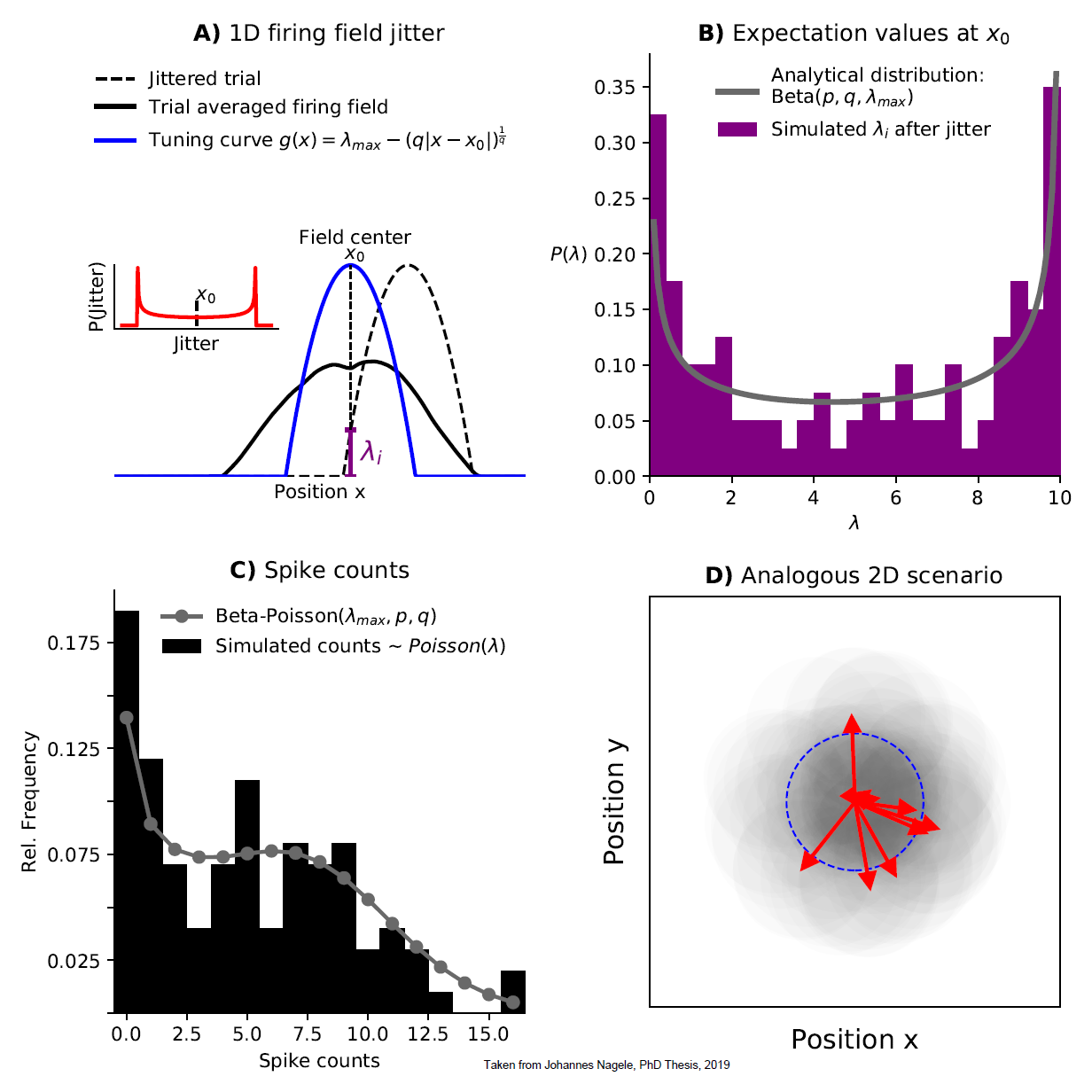
A jitter model leading to the Beta-Poisson spiking model.

A: Simulated 1D trial displacement, drawn from the jitter distribution in the inset ($P(jitter)\propto g(x)^{p-1}$). The trial-averaged firing field (solid black line) is broader and has a lower peak rate as compared to the underlying tuning curve without jitter (solid blue line, parameters used: $\lambda_{max} = 10, p = .6, q=.5$. B: The resulting distribution of $\lambda$ at $x_0$ across N=100 trials and the analytical pdf of the Beta distribution. C: Simulated spike count distribution from a Poisson process with parameters $\lambda_i$ where i denote the indices of the trials and the resulting Beta-Poisson distribution as derived as sketched above. D: Analogous situation in 2D with random shift angles leading to the identical statistics.

$\endgroup$

Your Answer

By clicking “Post Your Answer”, you agree to our terms of service and acknowledge you have read our privacy policy.

Not the answer you're looking for? Browse other questions tagged or ask your own question.