The fundamental theorem of simulation

Question

The Fundamental Theorem of Simulation

Simulating $X \sim f$

is equivalent to simulating

$(X,U) \sim \mathscr{U}\{(x,u): 0<u<f(x)\}$

The proof is trivial.

One thing that is made clear by this theorem is that we can generate X in three ways:

1. first generate $X \sim f$, and then $U|X=x$, but this is useless because we already have $X$ and don't need $X$
2. first generate $U$, and then $X|U=u$, that is just the accept-reject algorithm
3. generate $(X,U)$ jointly, which will eventually turn out be the smart idea because it allows us to generate data on a larger set were simulation is easier, and then to use the pair if the constraint is satisfied. http://academic.uprm.edu/wrolke/esma5015/fund.htm

I want to understand in last step,

we will sample $X$ using any method of MCMC and $U \sim U[0,1]$ and then take the sample of $X$ only which interested to find distribution for it.

Another question, Is this theorem related to latent variables?

Answer 1

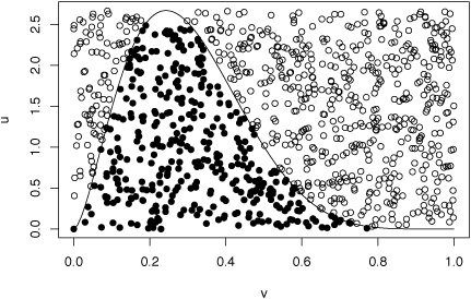
Your question is unclear: when simulating $X\sim f(x)$, one can instead simulate$$(X,U)\sim\mathcal{U}(\{(x,u);\ 0<u<f(x)\})$$which has the joint density$$\mathbb{I}_{(0,f(x)}(u)\mathbb{I}_\mathcal{X}(x)$$and then use only the $X$ component in the simulation. For instance, here is a figure from our book depicting many realisations of such a Uniform when $f$ is the density of a Beta distribution [black dots]. The remaining dots are rejected simulations from a Uniform over a square that contains the subgraph of $f$.

Once this new target is set, any simulation method aimed at it is valid. Like Accept-Reject in the above picture. What matters is to find an efficient simulation method. (The quote is then wrong in that $U$ is no longer $\mathcal{U}(0,1)$

As to your second question, the $U$ component in the above indeed behaves like a latent variable in the sense that $$f(x)=\int_0^\infty f(x,u)\text{d}u$$ represents the density of interest as the marginal density of a joint distribution of $(X,U)$, $U$ being "unobserved". However, latent variables are most often used in statistical settings where the joint $f(x,u)$ makes life easier, for instance allowing for an EM algorithm. In that sense $U$ is not a latent variable since this is not a statistical problem but a simulation problem. I would use "auxiliary" rather than "latent".