1
$\begingroup$

I'm sure this is dreadfully simple to everyone who sees it, but I'm completely lost. From what I've read, I think this concept must be so fundamental to Bayesian statistics that no one bothers to explain it. Anyway, here's a concept I'm trying to understand from a class:

I want to find the marginal distribution $f(x)=\int f(x|p)f(p)dp$ given $x|p\sim Binom(n,p)$ and $p\sim Beta(\alpha,\beta)$.

Then I want to get some summary statistics by drawing a few (hundreds) $x$ from $f(x)$ using an MCMC method. However, I must first draw a $p$ from $f(p)$ to draw an $x$ from $f(x)$.

My problem is these two points:

  1. $f(x)$ is not a distribution. It is the beta function and evaluates to $\frac{\Gamma(x+\alpha)\Gamma(n+\beta-y)}{\Gamma(\alpha+\beta+n)}$.
  2. There is no $p$ in the above $f(x)$ because I specifically integrated it out.

Even if I were to draw some $p$ from $f(p)$ there is no place for it in the beta function for it. In my understanding when doing this kind of sampling, my marginal distribution should be some kind of function (in this case since $P\sim Beta$, then $f(p)=p^{\alpha-1}(1-p)^{\beta-1}$) and then I draw the needed parameter ($p$) from its distribution (assuming $\alpha$ and $\beta$ are known) and plug it in to obtain my $x$.

Every resource I've seen up till now seems to only be dealing with posterior distributions, not this kind of integrated marginal distribution and none seem to deal with a sampling problem that does not contain the parameter I need to first sample for.

So why then do I need to draw the parameter for a marginal distribution that does not contain the parameter?


Major edit for clarification (My previous understanding of the concept was wrong):

I am trying to get the marginal distribution $f(x)=\int f(x|p)f(p)dp$, so I can calculate the statistics of $f(x)$ (e.g., mean). There are two ways to do so:

  1. Multiply and integrate the two distributions and then find the expectation. The result of this is and is supposed to be some $f(x)=$ equation with $x$ as an independent variable.
  2. Use sampling to generate a set of $x$ drawn from $f(x)$ by drawing $x$ from $f(x|p)$. To draw from $f(x|p)$ I first need a parameter $p$.

Example to draw 1000 samples:

list of samples $X=[x^{(1)},x^{(2)},...,x^{(1000)}]$.

$x^{(1)}\sim Binom(n,p)$ where $p\sim Beta(\alpha,\beta)$

$x^{(2)}\sim Binom(n,p)$ where $p\sim Beta(\alpha,\beta)$

...

To show it in simple R code:

a=1;b=1;n=50   #My arbitrary distribution parameters
X=double(1000) #An empty vector for X
for (i in seq(1,1000)){
  p = rbeta(1,a,b)
  X[i] = rbinom(1,n,p)
}
mean(X)

This is how to draw parameters to draw from a marginal distribution. I'll leave this here if I can, since I could not find anything online to explain it.

$\endgroup$
1
  • $\begingroup$ This follows from the definition of the marginal distribution as marginal of the joint. What is unclear about this notion? $\endgroup$
    – Xi'an
    Commented Oct 8, 2019 at 8:06

2 Answers 2

1
$\begingroup$

Let's first distinguish the prior $\pi(p)$ from the likelihood function $f(x|p)$ for clarity. Let the marginal likelihood (equivalently evidence, normalizing constant) $$f(x) = \int f(x|p) \pi(p)dp.$$

Before we do any drawing, let's consider what the model tells us.

$$p\sim\text{Beta}(\alpha,\beta)\\ y \sim \text{Binom}(n, p)$$

What this says is, we posit our observed data $y'$ is generated by first drawing a $p'$ from a Beta($\alpha, \beta$) distribution, then drawing a $y$ from a Binomial distribution with parameters $n,p'$.

After we perform our posterior inference, we obtain a posterior distribution $\pi(\cdot|x)$ over $p$. That is, a distribution over $p$ that takes into account our previous knowledge (prior) and information gained from new observations (likelihood function).

Now how do we draw new $x$'s from this updated model? Similar to before, we draw $p''$ from $\pi(\cdot|x)$, then draw $x''$ from a Binomial distribution with parameter $p''$. Repeat this multiple times for as many samples as you want.

-- summary --

The posterior distribution $\pi(\cdot|x)$ is a distribution over $p$. In some sense, it is your prior distribution upgraded.

You are correct, the marginal likelihood $f(x)$ is not a distribution. It is a constant: the probability of observing your data under this model.

To generate samples from your updated model, you draw a parameter from your posterior distribution, then draw $x$ from your sampling distribution parameterized by the new parameter you just drew.

--

Posterior distribution $$\pi( p | x ) = \frac{f(x|p) \pi(p)}{\int f(x|p) \pi(p) dp}$$

$\endgroup$
3
  • $\begingroup$ So you're saying the point of drawing $p'$ from $p$ is to get $y'$ from $y$ so that you can determine an observation for $f(x|p)$? Then you could get a $\pi(|x)$. Or, that would make sense without the integral, but with it the beta distribution of $\pi(|x)$ still becomes this non-distribution I have written above. $\endgroup$ Commented Oct 6, 2019 at 20:04
  • $\begingroup$ You obtain $x$, some data from some source. You have some prior distribution over $p$. Combining your prior knowledge and new observed data, you obtain a posterior distribution. For whatever reason, you want to generate data like $x$, so you draw a $p'$ from your posterior, then draw a $x'$ from a binomial with this new $p'$. $\endgroup$
    – fool
    Commented Oct 6, 2019 at 20:08
  • $\begingroup$ You're welcome, I hope it really did help. It might help to write a short R/Python program to do some simulations for intuition. $\endgroup$
    – fool
    Commented Oct 6, 2019 at 20:37
4
$\begingroup$

If the question is about simulation, rather than Bayesian statistics, since the mcmc tag is (unnecessarily) used, the generation of more variates than needed is quite common in random variate generations and goes under different names, like auxiliary variable models, latent variable models, demarginalisation, &tc.

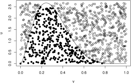
enter image description here

For instance, the generic accept-reject algorithm is based on a marginalisation argument, namely that the marginal distribution (in X) of the Uniform distribution on the sub-graph of $f$: $$\mathfrak S_f=\{(x,u);\ 0\le u\le f(x)\}$$ is the distribution with density proportional to $f$. This means that to produce an $X\sim f(x)$ one generates both $U$ and $X$, even though $U$ is not used as such and obviously does not appear in the (marginal) distribution of $X$. The accept-reject algorithm generates $(X,U)$ in a larger subgraph like the box in the image above and only keeps the $(X,U)$'s that fall under the curve $f$, i.e. in $\mathfrak S_f$.

In the current case, generating from a joint density $f(x|p)f(p)$ to produce simulations from$$m(x) = \int f(x|p)f(p)\,\text{d}p$$is another type of standard approach to the simulation of complex distributions and follows from the argument that if $(X,P)\sim f(x|p)f(p)$ then $X\sim m(x)$. This is the very definition of the marginal distribution but can also be seen by the "law of the unconscious statistician": $$\mathbb E[h(X)]=\int_{\mathcal X} h(x) m(x)\,\text{d}x = \int_{\mathcal X \times \mathcal P} h(x) f(x|p)f(p)\,\text{d}p\,\text{d}x$$ in that $h(x)$ is a function of $(x,p)$ that is constant in $p$.

$\endgroup$

Your Answer

By clicking “Post Your Answer”, you agree to our terms of service and acknowledge you have read our privacy policy.

Not the answer you're looking for? Browse other questions tagged or ask your own question.