LASSO for unit norm parameters?

Question

I have the model $y = X\theta +e$, where $\vert\vert \theta\vert\vert =1$ and $e$ are iid normal errors and $\vert\vert\cdot\vert\vert$ represents the Euclidean norm. Can I use a LASSO penalty in this case too? If so, does the fact that the parameters have a unit norm change the approach?

Answer 1

The problem is valid and can be solved by Projected Gradient Descent, where we project the solution to L2 ball constraint. Check my answer here for details.

In Projected Gradient Decent, the projection step is another optimization problem.In this problem, we want to find a point in $C$ (constraint set), this point is closest to a given point $x^*$. Which is $$ \underset{x \in C}{\text{arg min}} \|x-x^*\| $$

In certain cases, this optimization problem is easy to solve and have closed from for example, box constraint or L2 ball. For L2 ball, the solution is:

$$ \underset{x \in C}{\text{arg min}} \|x-x^*\|=\left\{ \begin{array}{ll} x^* & \|x^*\| \leq r \\ r \frac {x^*} {\|x\|} & \text{otherwise} \\ \end{array} \right. $$

The equation tells, if the point is inside of the constraint domain, then the projection is the point itself.

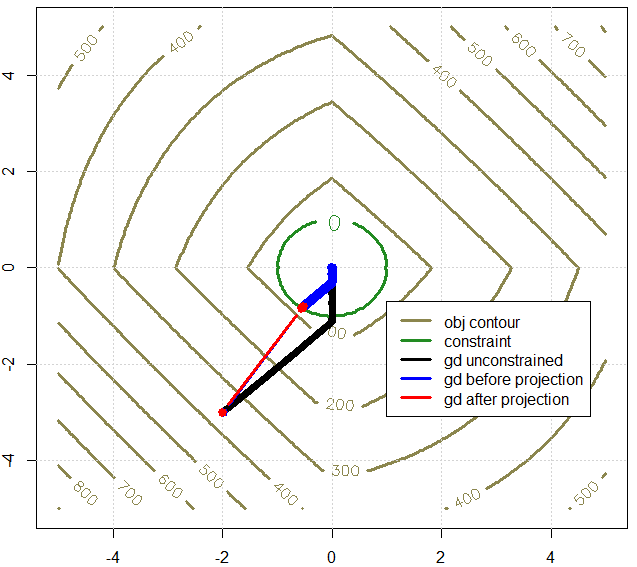
And I will demonstrate the $r \frac {x^*} {\|x\|}$ case graphically, check the points (labeled with numbers) in blue track and red track, the relationship is easy: connect the blue dots with the center of the circle, the intersection with the circle is the projection.

The following figure gives how it works visually: where the red trace is projected gradient decent trace. In the experiment, I set a large $\lambda$ on L1 regularization, and the optimal point is close to the origin. We can clear see the projected solution (red dots) is on the unit circle.

PS: R code if you want to experiment more.

---

fn<-function(x,A,b,l1,l2){
  e=A %*% x - b
  v=crossprod(e)+l2*crossprod(x)+l1*sum(abs(x))
  return(c(v))
}

gr<-function(x,A,b,l1,l2){
  v=t(A) %*% (A %*% x -b)
  return(2*c(v)+2*l2*x+l1*sign(x))
}

set.seed(0)
par(cex=1)
n_data=10
n_feature=2

A=matrix(runif(n_data*n_feature),ncol=n_feature)
b=matrix(runif(n_data),ncol=1)

l1=50
l2=0

# plot obj function
x1=seq(-5,5,0.05)
x2=seq(-5,5,0.05)
d=expand.grid(x1,x2)
f_v=matrix(apply(d,1,fn, A=A, b=b, l1=l1 , l2=l2),nrow=length(x1))
contour(x1,x2,f_v, lwd=3, labcex=1,col='khaki4', xlim=c(-5,5),ylim=c(-5,5))
grid()
constraint_v=outer(x1,x2,function(x,y) x^2+y^2-1)
contour(x1,x2,constraint_v, lwd=3, levels=0, add=T,col="forestgreen",labcex=1.5)

# solve the unconstrained optimization using toolbox
opt_res=optimx::optimx(c(-1,-1),fn, gr, method="BFGS", A=A, b=b, l1=l1 , l2=l2)
opt_x=c(opt_res$p1,opt_res$p2)
points(opt_x[1],opt_x[2],pch=19,col="black")

#-------------------------------------------------------------------
# all algorithms fix step size
# solve unconstrained optimization using gradient decent
x_init=c(-2,-3)
t=0.0001
f_opt=opt_res$value
x=x_init
trace_x=x_init
while(fn(x, A, b, l1 , l2)- f_opt> 1e-2){
  x=x-t*gr(x, A=A, b=b, l1=l1 , l2=l2)
  trace_x=rbind(trace_x,x)
  print(x)
}
# for GD we just plot points not string labels
points(trace_x,type='b',pch=19)


# solve constrained optimization using projected gradient decent
# x_d means desired place to go, x means after projection
x_init=c(-2,-3)
t=0.0001
x=x_init
f_opt=opt_res$value
trace_x=x_init
trace_x_d=x_init

while(fn(x, A, b, l1 , l2)-f_opt>1e-2){
  x_d=x-t*gr(x, A=A, b=b, l1=l1 , l2=l2)
  trace_x_d=rbind(trace_x_d,x_d)

  if(norm(x_d,'2')<1){
    x=x_d
  }
  else{
    x=1*x_d/norm(x_d,'2')
  }
  trace_x=rbind(trace_x,x)
}
trace_x=head(trace_x)
trace_p=head(trace_x_d)

points(trace_x_d,type='b',col=4,pch=19,lwd=3)
points(trace_x,type='b',col=2,pch=19,lwd=3)


legend(1,-0.7,c('obj contour','constraint', 'gd unconstrained',
                 'gd before projection', 'gd after projection'),
       lwd=3,col=c("khaki4",'forestgreen','black','blue','red'))

Answer 2

This can likely be solved with the elastic net. Suppose we have response $y \in \mathbb{R}^n$ and design matrix $X \in \mathbb{R}^{n \times p}$.

By lagrangian duality, the estimator $$\hat\theta_{(a)} = \arg\min_{\theta \in \mathbb{R}^p \, : \, \|\theta\|_1 \leq C_1, \, \|\theta\|_2 \leq 1} \|y-X\theta\|_2^2$$ is also the minimizer $$\hat\theta_{(b)} = \arg\min_{\theta \in \mathbb{R}^p} \frac{1}{2n} \|y - X \theta\|_2^2 + \lambda \|\theta\|_1 + \mu \|\theta\|_2^2$$ for some dual variables $\lambda$ and $\mu$. That is, $\hat\theta_{(a)} = \hat\theta_{(b)} \left( =: \hat\theta \right)$. That means that all you have to do is tune $\mu$ appropriately to achieve the desired $\ell_2$ norm of the estimate $\hat\theta_{(b)}$. Further, you have to be sure that $\lambda$ is not "too large" to ensure that there exists some $\mu$ so that the estimate $\hat\theta_{(b)}$ can have $\ell_2$ norm equal to one.

The only hitch here is that the estimator you are actually interested in is $$\tilde\theta = \arg\min_{\theta \in \mathbb{R}^p \, : \, \|\theta\|_1 \leq C_1, \, \|\theta\|_2 = 1} \|y-X\theta\|_2^2,$$ and it isn't necessarily true that $\hat\beta = \tilde\beta$. However, we can see that $\tilde\theta = \hat\theta$ if $\mu \ne 0$ by complementary slackness. (Notice, of course, that this $\mu$ was specifically defined to be the dual variable corresponding to the bound of $1$--it isn't arbitrary.) In general though, it's possible that $\|\hat\theta_{(b)} \|_2 > 1$ for all possible choices of $(\lambda, \mu)$. In which case, the problem you're trying to solve is nonconvex and elastic net would not work: you'd have to do a more complicated optimization method, perhaps like hxd mentions.

It's also worth pointing out that $\|\hat\theta_{(b)}\|_2$ is not necessarily monotonically decreasing with respect to $\lambda$. See, for instance, Can $\|\beta^*\|_2$ increase when $\lambda$ increases in Lasso?.