72
$\begingroup$

This question is motivated by my question on meta-analysis. But I imagine that it would also be useful in teaching contexts where you want to create a dataset that exactly mirrors an existing published dataset.

I know how to generate random data from a given distribution. So for example, if I read about the results of a study that had:

  • a mean of 102,
  • a standard deviation of 5.2 , and
  • a sample size of 72.

I could generate similar data using rnorm in R. For example,

set.seed(1234)
x <- rnorm(n=72, mean=102, sd=5.2)

Of course the mean and SD would not be exactly equal to 102 and 5.2 respectively:

round(c(n=length(x), mean=mean(x), sd=sd(x)), 2)
##     n   mean     sd 
## 72.00 100.58   5.25 

In general I'm interested in how to simulate data that satisfies a set of constraints. In the above case, the constaints are sample size, mean, and standard deviation. In other cases, there might be additional constraints. For example,

  • a minimum and a maximum in either the data or the underlying variable might be known.
  • the variable might be known to take on only integer values or only non-negative values.
  • the data might include multiple variables with known inter-correlations.

Questions

  • In general, how can I simulate data that exactly satisfies a set of constraints?
  • Are there articles written about this? Are there any programs in R that do this?
  • For the sake of example, how could and should I simulate a variable so that it has a specific mean and sd?
$\endgroup$
13
  • 1
    $\begingroup$ Why do you want them to be exactly like the published results? Aren't these estimates of the population mean and standard deviation given their sample of data. Given uncertainty in those estimates, who is to say that the sample you show above is not consistent with their observations? $\endgroup$ Commented Jun 12, 2012 at 11:21
  • 5
    $\begingroup$ Because this question appears to be collecting replies that miss the mark (IMHO), I would like to point out that conceptually the answer is straightforward: equality constraints are treated like marginal distributions and inequality constraints are multivariate analogs of truncation. Truncation is relatively easy to handle (often with rejection sampling); the harder problem amounts to finding a way to sample these marginal distributions. This means either sampling marginals given the distribution and the constraint, or integrating to find the marginal distribution and sampling from it. $\endgroup$
    – whuber
    Commented Jun 12, 2012 at 14:07
  • 6
    $\begingroup$ BTW, the last question is trivial for location-scale distribution families. E.g., x<-rnorm(72);x<-5.2*(x-mean(x))/sd(x)+102 does the trick. $\endgroup$
    – whuber
    Commented Jun 12, 2012 at 14:48
  • 1
    $\begingroup$ @whuber, as cardinal alludes to in a comment to my answer (which mentions this "trick") and a comment to another answer - this method, in general, will not keep the variables within the same distributional family, since you're dividing by the sample standard deviation. $\endgroup$
    – Macro
    Commented Jun 12, 2012 at 15:04
  • 6
    $\begingroup$ @Macro This is a good point, but perhaps the best reply is, "of course they won't have the same distribution"! The distribution you want is the distribution conditional on the constraints. In general that will not be from the same family as the parent distribution. E.g., each element of a sample of size 4 with mean 0 and SD 1 drawn from a normal distribution is going to have nearly a uniform probability on [-1.5, 1.5], because the conditions place upper and lower bounds on the possible values. $\endgroup$
    – whuber
    Commented Jun 12, 2012 at 15:33

8 Answers 8

32
$\begingroup$

In general, to make your sample mean and variance exactly equal to a pre-specified value, you can appropriately shift and scale the variable. Specifically, if $X_1, X_2, ..., X_n$ is a sample, then the new variables

$$ Z_i = \sqrt{c_{1}} \left( \frac{X_i-\overline{X}}{s_{X}} \right) + c_{2} $$

where $\overline{X} = \frac{1}{n} \sum_{i=1}^{n} X_i$ is the sample mean and $ s^{2}_{X} = \frac{1}{n-1} \sum_{i=1}^{n} (X_i - \overline{X})^2$ is the sample variance are such that the sample mean of the $Z_{i}$'s is exactly $c_2$ and their sample variance is exactly $c_1$. A similarly constructed example can restrict the range -

$$ B_i = a + (b-a) \left( \frac{ X_i - \min (\{X_1, ..., X_n\}) }{\max (\{X_1, ..., X_n\}) - \min (\{X_1, ..., X_n\}) } \right) $$

will produce a data set $B_1, ..., B_n$ that is restricted to the interval $(a,b)$.

Note: These types of shifting/scaling will, in general, change the distributional family of the data, even if the original data comes from a location-scale family.

Within the context of the normal distribution the mvrnorm function in R allows you to simulate normal (or multivariate normal) data with a pre-specified sample mean/covariance by setting empirical=TRUE. Specifically, this function simulates data from the conditional distribution of a normally distributed variable, given the sample mean and (co)variance is equal to a pre-specified value. Note that the resulting marginal distributions are not normal, as pointed out by @whuber in a comment to the main question.

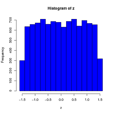
Here is a simple univariate example where the sample mean (from a sample of $n=4$) is constrained to be 0 and the sample standard deviation is 1. We can see that the first element is far more similar to a uniform distribution than a normal distribution:

library(MASS)
 z = rep(0,10000)
for(i in 1:10000)
{
    x = mvrnorm(n = 4, rep(0,1), 1, tol = 1e-6, empirical = TRUE)
    z[i] = x[1]
}
hist(z, col="blue")

$ \ \ \ \ \ \ \ \ \ \ \ \ \ \ \ \ \ $ enter image description here

$\endgroup$
11
  • 1
    $\begingroup$ The $Z_i$ will not be normally distributed, though they may be approximately so if the sample size is large. The first comment to @Sean's answer alludes to this. $\endgroup$
    – cardinal
    Commented Jun 12, 2012 at 14:14
  • 1
    $\begingroup$ Well, that's a pretty natural thing to want to do...and oftentimes doesn't cause too much trouble. $\endgroup$
    – cardinal
    Commented Jun 12, 2012 at 14:23
  • 1
    $\begingroup$ +1. In the example, the uniform is the exact answer, by the way. (The apparent dropoff at the ends of the plot is an artifact of how R draws histograms.) $\endgroup$
    – whuber
    Commented Jun 12, 2012 at 23:16
  • 1
    $\begingroup$ @whuber, thanks for motivating this example. Given the fact that the marginal distributions change once you condition on the sample mean/variance, it seems that the best "answer" in the spirit of the OP's question is just to simulate data with population mean/variance equal to that reported as the sample quantities (as suggested by the OP himself), doesn't it? That way, you get sample quantities "similar" to those desired, and the marginal distributions are what you wanted them to be. $\endgroup$
    – Macro
    Commented Jun 12, 2012 at 23:21
  • 1
    $\begingroup$ @whuber, If your sample is normal, then $T_i = (X_i-\overline{X})/s$ has a $t$-distribution, yes? The "new" variable in question will just be a linear combination of $T_i$. $\endgroup$
    – Macro
    Commented Jun 12, 2012 at 23:35
28
$\begingroup$

Regarding your request for papers, there is:

This isn't quite what you're looking for, but might serve as grist for the mill.


There is another strategy that no one seems to have mentioned. It is possible to generate $N-k$ (pseudo) random data out of a set of size $N$ such that whole set meets $k$ constraints so long as the remaining $k$ data are fixed at appropriate values. The required values should be solvable with a system of $k$ equations, algebra, and some elbow grease.

For example, to generate a set of $N$ data from a normal distribution that will have a given sample mean, $\bar x$, and variance, $s^2$, you will need to fix the values of two points: $y$ and $z$. Since the sample mean is:
$$ \bar x = \frac{\sum_{i=1}^{N-2}x_i\; + \;y\!+\!z}{N} $$ $y$ must be: $$ y = N\bar x\; - \;\left(\sum_{i=1}^{N-2}x_i\!+\!z\right) $$ The sample variance is: $$ s^2 = \frac{\sum_{i=1}^{N-2}(x_i - \bar x)^2\; + \;(y - \bar x)^2\!+\!(z - \bar x)^2}{N-1} $$ thus (after substituting the above for $y$, foiling / distributing, & rearranging...) we get: $$ 2(N\bar{x}\! - \!\sum_{i=1}^{N-2}x_i)z - 2z^2 = N\bar{x}^2(N\!-\!1) + \sum_{i=1}^{N-2}x_i^2 + \left[\sum_{i=1}^{N-2}x_i\right]^2 - 2N\bar{x}\sum_{i=1}^{N-2}x_i - (N\!-\!1)s^2 $$ If we take $a=-2$, $b=2(N\bar{x} - \sum_{i=1}^{N-2}x_i)$, and $c$ as the negation of the RHS, we can solve for $z$ using the quadratic formula. For example, in R, the following code could be used:

find.yz = function(x, xbar, s2){
  N    = length(x) + 2
  sumx = sum(x)
  sx2  = as.numeric(x%*%x)          # this is the sum of x^2
  a    = -2
  b    = 2*(N*xbar - sumx)
  c    = -N*xbar^2*(N-1) - sx2 - sumx^2 + 2*N*xbar*sumx + (N-1)*s2
  rt   = sqrt(b^2 - 4*a*c)

  z    = (-b + rt)/(2*a)
  y    = N*xbar - (sumx + z)
  newx = c(x, y, z)
  return(newx)
}

set.seed(62)
x    = rnorm(2)
newx = find.yz(x, xbar=0, s2=1)
newx                                # [1] 0.8012701  0.2844567  0.3757358 -1.4614627
mean(newx)                          # [1] 0
var(newx)                           # [1] 1

There are some things to understand about this approach. First, it's not guaranteed to work. For example, it is possible that your initial $N-2$ data are such that no values $y$ and $z$ exist that will make the variance of the resulting set equal $s^2$. Consider:

set.seed(22)    
x    = rnorm(2)
newx = find.yz(x, xbar=0, s2=1)
Warning message:
In sqrt(b^2 - 4 * a * c) : NaNs produced
newx                                # [1] -0.5121391  2.4851837        NaN        NaN
var(c(x, mean(x), mean(x)))         # [1] 1.497324

Second, whereas standardizing makes the marginal distributions of all your variates more uniform, this approach only affects the last two values, but makes their marginal distributions skewed:

set.seed(82)
xScaled = matrix(NA, ncol=4, nrow=10000)
for(i in 1:10000){
  x           = rnorm(4)
  xScaled[i,] = scale(x)
}
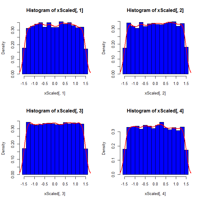
(insert plot)

set.seed(82)
xDf = matrix(NA, ncol=4, nrow=10000)
i   = 1
while(i<10001){
  x       = rnorm(2)
  xDf[i,] = try(find.yz(x, xbar=0, s2=2), silent=TRUE)  # keeps the code from crashing
  if(!is.nan(xDf[i,4])){ i = i+1 }                      # increments if worked
}
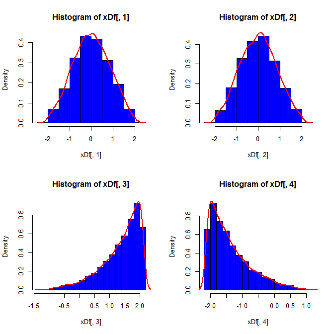
(insert plot)

Third, the resulting sample may not look very normal; it might look like it has 'outliers' (i.e., points that come from a different data generating process than the rest), since that is essentially the case. This is less likely to be a problem with larger sample sizes, as the sample statistics from the generated data should converge to the required values and thus need less adjustment. With smaller samples, you could always combine this approach with an accept / reject algorithm that tries again if the generated sample has shape statistics (e.g., skewness and kurtosis) that are outside of acceptable bounds (cf., @cardinal's comment), or extend this approach to generate a sample with a fixed mean, variance, skewness, and kurtosis (I'll leave the algebra up to you, though). Alternatively, you could generate a small number of samples and use the one with the smallest (say) Kolmogorov-Smirnov statistic.

library(moments)
set.seed(7900)  
x = rnorm(18)
newx.ss7900 = find.yz(x, xbar=0, s2=1)
skewness(newx.ss7900)                       # [1] 1.832733
kurtosis(newx.ss7900) - 3                   # [1] 4.334414
ks.test(newx.ss7900, "pnorm")$statistic     # 0.1934226

set.seed(200)  
x = rnorm(18)
newx.ss200 = find.yz(x, xbar=0, s2=1)
skewness(newx.ss200)                        # [1] 0.137446
kurtosis(newx.ss200) - 3                    # [1] 0.1148834
ks.test(newx.ss200, "pnorm")$statistic      # 0.1326304 

set.seed(4700)  
x = rnorm(18)
newx.ss4700 = find.yz(x, xbar=0, s2=1)
skewness(newx.ss4700)                       # [1]  0.3258491
kurtosis(newx.ss4700) - 3                   # [1] -0.02997377
ks.test(newx.ss4700, "pnorm")$statistic     # 0.07707929S
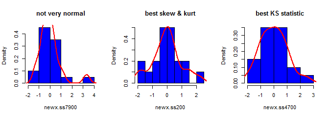
(add plot)

$\endgroup$
11
$\begingroup$

Are there any programs in R that do this?

The Runuran R package contains many methods for generating random variates. It uses C libraries from the UNU.RAN (Universal Non-Uniform RAndom Number generator) project. My own knowledge of the field of random variate generation is limited, but the Runuran vignette provides a nice overview. Below are the available methods in the Runuran package, taken from the vignette:

Continuous distributions:

  • Adaptive Rejection Sampling
  • Inverse Transformed Density Rejection
  • Polynomial Interpolation of Inverse CDF
  • Simple Ratio-of-Uniforms Method
  • Transformed Density Rejection

Discrete distributions:

  • Discrete Automatic Rejection Inversion
  • Alias-Urn Method
  • Guide-Table Method for Discrete Inversion

Multivariate distributions:

  • Hit-and-Run algorithm with Ratio-of-Uniforms Method
  • Multivariate Naive Ratio-of-Uniforms Method

Example:

For a quick example, suppose you wanted to generate a Normal distribution bounded between 0 and 100:

require("Runuran")

## Normal distribution bounded between 0 and 100
d1 <- urnorm(n = 1000, mean = 50, sd = 25, lb = 0, ub = 100)

summary(d1)
sd(d1)
hist(d1)

The urnorm() function is a convenient wrapper function. I believe that behind the scenes it uses the Polynomial Interpolation of Inverse CDF method but am not sure. For something more complex, say, a discrete Normal distribution bounded between 0 and 100:

require("Runuran")

## Discrete normal distribution bounded between 0 and 100
# Create UNU.RAN discrete distribution object
discrete <- unuran.discr.new(pv = dnorm(0:100, mean = 50, sd = 25), lb = 0, ub = 100)

# Create UNU.RAN object using the Guide-Table Method for Discrete Inversion
unr <- unuran.new(distr = discrete, method = "dgt")

# Generate random variates from the UNU.RAN object
d2 <- ur(unr = unr, n = 1000)

summary(d2)
sd(d2)
head(d2)
hist(d2)
$\endgroup$
10
$\begingroup$

The general technique is the 'Rejection Method', where you just reject results that don't meet your constraints. Unless you have some sort of guidance (like MCMC), then you could be generating a lot of cases (depending on your scenario) which are rejected!

Where you're looking for something like a mean and standard deviation and you can create a distance metric of some kind to say how far you are away from your goal, you can use optimisation to search for the input variables which give you the desired output values.

As an ugly example where we will look for a random uniform vector with length 100 which has mean=0 and standard deviation=1.

# simplistic optimisation example
# I am looking for a mean of zero and a standard deviation of one
# but starting from a plain uniform(0,1) distribution :-)
# create a function to optimise
fun <- function(xvec, N=100) {
  xmin <- xvec[1]
  xmax <- xvec[2]
  x <- runif(N, xmin, xmax)
  xdist <- (mean(x) - 0)^2 + (sd(x) - 1)^2
  xdist
}
xr <- optim(c(0,1), fun)

# now lets test those results
X <- runif(100, xr$par[1], xr$par[2])
mean(X) # approx 0
sd(X)   # approx 1
$\endgroup$
3
  • 8
    $\begingroup$ Constraints that occur with probability zero are hard to satisfy. ;-) For the specific example at hand, an appropriate shift and dilation easily achieves the stated goals, though one might want to analyze a bit deeper to look at how the distribution of the data is perturbed by such an operation. $\endgroup$
    – cardinal
    Commented Jun 12, 2012 at 11:37
  • $\begingroup$ Thanks. Certainly it would be easy to reject observations less than the min and larger than the max. And I can see how you could define it as an optimisation problem. It would be great to see some examples or maybe have some suggestions of what to read next. $\endgroup$ Commented Jun 12, 2012 at 11:43
  • 1
    $\begingroup$ @cardinal - agreed. One should look at the distributions (i.e. a histogram) of both the input simulated numbers and output as sometimes these can look very strange indeed! $\endgroup$
    – Sean
    Commented Jun 12, 2012 at 11:43
3
$\begingroup$

It seems that there is an R package meeting your requirement published just yesterday! simstudy By Keith Goldfeld

Simulates data sets in order to explore modeling techniques or better understand data generating processes. The user specifies a set of relationships between covariates, and generates data based on these specifications. The final data sets can represent data from randomized control trials, repeated measure (longitudinal) designs, and cluster randomized trials. Missingness can be generated using various mechanisms (MCAR, MAR, NMAR).

$\endgroup$
1
  • 1
    $\begingroup$ Neither in the vignette nor on the program's home page exact meeting of constraints is mentioned. Why do you think this package meets the requirement of drawing from conditional distributions? $\endgroup$
    – g g
    Commented Apr 21, 2019 at 8:32
2
$\begingroup$

This is an answer coming so late it is presumably meaningless, but there is always an MCMC solution to the question. Namely, to project the joint density of the sample$$\prod_{i=1}^n f(x_i)$$on the manifold defined by the constraints, for instance $$\sum_{i=1}^n x_i=\mu_0\qquad\sum_{i=1}^n x_i^2=\sigma_0^2$$ The only issue is then in simulating values over that manifold, i.e., finding a parameterisation of the correct dimension. A 2015 paper by Bornn, Shephard and Solgi studies this very problem (with an interesting if not ultimate answer).

$\endgroup$
2
$\begingroup$

This answer considers another approach to the case where you want to force the variates to lie in a specified range and additionally dictate the mean and/or variance.

Restrict our attention to the unit interval $[0,1]$. Let's use a weighted mean for generality, so fix some weights $w_k\in[0,1]$ with $\sum_{k=1}^Nw_k=1$, or set $w_k=1/N$ if you want standard weighting. Suppose the quantities $\mu\in(0,1)$ and $0<\sigma^2<\mu(1-\mu)$ represent the desired (weighted) mean and (weighted) variance, respectively. The upper bound on $\sigma^2$ is necessary because that's the maximum variance possible on a unit interval. We are interested in drawing some variates $x_1,...,x_N$ from $[0,1]$ with these moment restrictions.

First we draw some variates $y_1,...,y_N$ from any distribution, like $N(0,1)$. This distribution will affect the shape of the final distribution. Then we constrain them to the unit interval $[0,1]$ using a logistic function:

$$ x_k=\frac{1}{1+e^{-(y_k v-h)}} $$

Before we do that, however, as seen in the equation above, we transform the $y_k$'s with the translation $h$ and scale $v$. This is analogous to the first equation in @Macro's answer. The trick is now to choose $h$ and $v$ so that the transformed variables $x_1,...,x_N$ have the desired moment(s). That is, we require one or both of the following to hold: $$ \mu=\sum_{k=1}^N \frac{w_k}{1+e^{-(y_k v-h)}} \\ \sigma^2=\sum_{k=1}^N \frac{w_k}{(1+e^{-(y_k v-h)})^2} - \left( \sum_{k=1}^N \frac{w_k}{1+e^{-(y_k v-h)}} \right)^2 $$

Inverting these equations for $v$ and $h$ analytically is not feasible, but doing so numerically is straight forward, especially since derivatives with respect to $v$ and $h$ are easy to compute; it only takes a few iterations of Newton's method.

As a first example, let's say we only care about constraining the weighted mean and not the variance. Fix $\mu=0.8$, $v=1$, $w_k=1/N$, $N=200000$. Then for the underlying distributions $N(0,1)$, $N(0,0.1)$ and $\text{Unif}(0,1)$ we end up with the following histograms, respectively, and such that the mean of the variates is exactly $0.8$ (even for small $N$):

Example1

Next, let's constrain both the mean and variance. Take $\mu=0.2$, $w_k=1/N$, $N=2000$ and consider the three desired standard deviations $\sigma=0.1,0.05,0.01$. Using the same underlying distribution $N(0,1)$, here are the histograms for each:

Example 2

Note that these may look a bit beta-distributed, but they are not.

$\endgroup$
1
$\begingroup$

In my answer here, I listed three R packages for doing this:

$\endgroup$
1
  • $\begingroup$ There must be some format for a link to references. Should it be a comment instead? $\endgroup$
    – abalter
    Commented Aug 13, 2019 at 20:15

Your Answer

By clicking “Post Your Answer”, you agree to our terms of service and acknowledge you have read our privacy policy.

Not the answer you're looking for? Browse other questions tagged or ask your own question.