glmer model convergence issues

Question

I've hunted around for the past few days for a possible solution to my problem, but haven't found any work-arounds thus far.

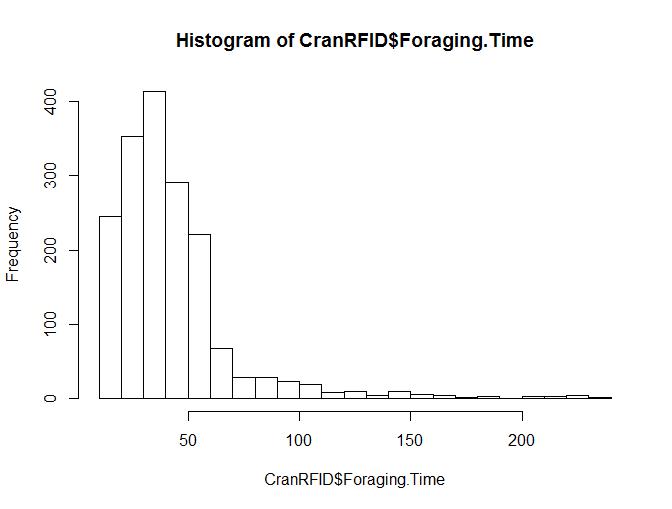
I have data that describe the foraging durations (in minutes) of an animal (continuous, repeated-measure response variable). Because these data are very right skewed (skewness measure using descdist() function = 2.918 - see histogram below) and highly peaked (kurtosis measure = 14.857 also from descdist() function), I'm interested in building a generalized linear mixed model using a gamma distribution with log-link function to test whether the foraging duration is different during three different time periods (variable called phenology: before, during, and after an environmental disturbance; a 3-level predictor).

I a couple other fixed-effects including year and landscape type, as well as the two-way interactions between time period, year, and landscape type as well as a suite of weather covariates, and then a random effect of the individual to account for the repeated measures (total of 100 individuals recorded). Overall, I've got 1754 unique foraging events, so a decent sized data set.

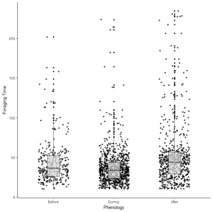
The data, when plotted, look like this (raw foraging times, plotted by phenological period):

Data example (made up, just to show structure):

Date    Year    Landscape.Type    Foraging.Time    Phenology    Indivivdual.ID
6/7/15  2015    Low Woodland      16.41            Before       03 BA 56 44
6/7/15  2015    Low Woodland      25.65            Before       03 BA 56 44
6/30/15 2015    High Woodland     19.56            During       04 BA 57 44
7/2/15  2015    High Woodland     23.45            During       04 BA 57 44
7/2/16  2016    Low Woodland      12.56            During       05 BA 56 00
7/19/16 2016    Low Woodland      45.85            After        05 BA 56 00
7/19/16 2016    High Woodland     52.78            After        08 AA 56 10

The model that I'm interested in constructing is (with weather covariates removed - those aren't causing the issues as far as I can tell):

glmer <- glmer(Foraging.Time ~ Phenology + Year + Landscape.Type + 
                   Phenology:Year + Phenology:Landscape.Type + Landscape.Type:Year + 
                   (1 | Individual.ID), data = df, 
                 family = Gamma(link = "log"))

When I run this, I get the following error:

In checkConv(attr(opt, "derivs"), opt$par, ctrl = control$checkConv,  :
Model failed to converge with max|grad| = 0.0484185 (tol = 0.001, component 1)

I've iteratively built the model one effect at a time, and it appears that the random effect of individual is what's giving the model trouble in converging, perhaps because there are 100 individuals? I've also tried the "bobyqa" optimizer and upping the max iterations, to no avail. Obviously retaining this random effect is essential given that individuals were repeatedly measured within each phenological period.

When I first set about building a model, I log-transformed the response variable to normalize, and then fit a linear mixed effects model using lmer. That worked out well and yielded a relatively well-fit model after examining diagnostic plots. It has been suggested by some reviewers of this analysis in a MS I have submitted that I try a GLMM instead (they didn't really provide any justification as to why I should use a GLMM in place of an lmm, but I assume to make parameter estimates easier to understand, avoid messing up variance by using log-transformed data).

Overall, I am looking if anyone has suggestions of different optimizers or ways to help my glmer model fit, or if you see any other issues that I'm not seeing. I've read through the ?convergence help document, and still don't quite know which possible methods I could try to get the model to fit. I don't think re-scaling variables will really help here as most of them are factors and not continuous (other than weather covariates).

Many thanks for any suggestions!

Answer 1

(this may be better as a comment than an answer, but I can't comment, so...)

I worked around a similar problem by using the option nAGQ=0 (see ?glmer) which implements a faster but less precise convergence method. See: GLMER not converging Check the suggestions in comments on that quetion too.

There are other packages in R that run GLMMs, some of which use different estimation methods, it may be worth giving one of these a try to see if it avoids the convergence problem. I am afraid I do not know enough to advise on the advantages and disadvantages of different convergence methods used by different packages (perhaps someone else may be along to comment on that aspect). However, this paper http://avesbiodiv.mncn.csic.es/estadistica/curso2011/regm26.pdf does give a run down of several availible methods with some of the +/- points of each (and corresponding packages in R). It is a little old now and there is at least one other new R package glmmTMB, that is not mentioned, but should serve as a starting point.