Eigen-vectors and skewness

Question

I'm doing some experiments to assess the extend to which MV skewed distributions can affect eigen-vectors (and more specifically Deming regressions).

Suppose $X=(x_i,...,x_n')$ with $x_i \in \mathbb{R}^p$, $1\leq i \leq n$ and for simplicity $p=2$.

I'll be using a (univariate) measure of directional scatter that does not assume symmetricity ($\alpha\in \mathbb{R}^p:||\alpha||=1$):

$$\text{IQR}(X'\alpha)\;\;\;[1]$$

Now, suppose we are trying to find $\alpha^*$:

$$\alpha^*=\underset{\alpha\in \mathbb{R}^p:||\alpha||=1}{\text{Arg.min.}}\;\;\;\text{IQR}(X'\alpha)\;\;\;[2]$$

Then, we have (at least, more suggestions are welcomed) two alternative strategies for finding $\alpha^*$:

• (a) Sample (pseudo-randomly) a large number $M$ ($M=1000$) of $\alpha_i$'s from the appropriate space$^0$, for each $\alpha_i$ compute $[1]$ and retain as $\alpha^*$ the one that minimizes $[2]$.
• (b) Use as $\alpha^*$ the eigen-vector corresponding to the last eigen-value of the variance-covariance matrix of $X$.

These two strategies should --for large enough $M$ and $n$-- give comparable results when the $X$'s have an elliptical density, but notice that only strategy (b) requires the elliptical assumption.

Now, i'm trying to measure the difference between the two approaches on skewed $X$ to assess the extend to which skweness affects the estimation of the last eigen-vector --i'm really interested in the consequence of skewness, so i'll only use distributions with finite second moments.

I've tried two (simple) bivariate skewed distributions for the $X$ (the skew normal and the log-normal$^1$) and i don't find large differences $^2$ between approach (a) and (b).

This, and some thinking, lead me to conclude that it's hard to imagine a skewness mechanism that would make (a) very different from (b). I was wondering whether anyone here has a counter-example to that?

$^0$that is, the $\alpha_m$ are the directions of the hyperplanes through $p$ points drawn equiprobably from $1:n$;

$^1$I coordinate-wise $\exp$-ed a MV Gaussian centered at the origin with component-wise variances less than 2 to avoid numerical troubles.

$^2$the median differences over 100 trials are about 10%, which is not very much considering the low efficiency of the IQR.

Answer 1

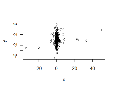
The IQR captures the middle 50% of a distribution. The variance-covariance matrix records second moments, which we can think of as weighted averages of values--with the weights given by the values themselves. Thus a few extreme values will influence the latter while having little or no influence on the former. These two characterizations suggest we can construct a counterexample by combining a distribution that is narrow along the middle 50% of its values with one that has a small proportion of extraordinarily large values. Do this along one axis and along all axes orthogonal to it, do something "tame."

Thus:

set.seed(17)
n <- 100               # Number of small values in the x direction
m <- 80                # Number of potentially large values in the x direction
x <- c(runif(n, min=-1/2, max=1/2), 1/rnorm(m))
y <- rnorm(n+m, sd=2)  # Intermediate values go in the y direction
data <- cbind(x,y)     # Create (x,y) data
plot(data)
cov(data)
eigen(cov(data))
c(IQR(x), IQR(y))

The eigenvectors, which are close to $(-1,0)$ and $(0,-1)$, show that the principal directions are essentially $(1,0)$ and $(0,1)$. The eigenvalues indicate there is much less variance along the latter direction (4.1 vs 38.2). However, the IQR along the first principal direction (0.86) is only about a third of that along the second direction (2.6), exactly as planned. Although this does not exactly determine $\alpha^*$, I hope it makes it clear why $\alpha^*$ and the smallest principal direction can be arbitrarily far apart.

These data can be made "skew" in the technical sense (of a substantial standardized third central moment) simply by extending some of the extreme $x$ values on one side of the plot compared to the other. This will barely change the eigenvectors or the IQRs.