What's the distribution of these data?

Question

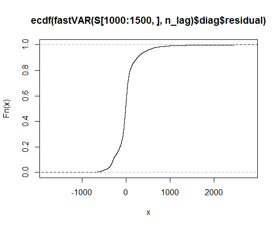
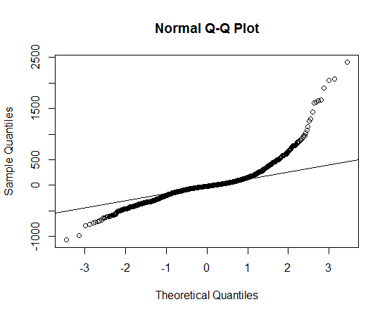
I got the data, and plot the distribution of the data, and use the qqnorm function, but is seems doesn't follow a normal distribution, so which distribution should I use to discribe the data?

Empirical cumulative distribution function

Answer 1

I suggest you give heavy-tail Lambert W x F or skewed Lambert W x F distributions a try (disclaimer: I am the author). In R they are implemented in the LambertW package.

They arise from a parametric, non-linear transformation of a random variable (RV) $X \sim F$, to a heavy-tailed (skewed) version $Y \sim \text{Lambert W} \times F$. For $F$ being Gaussian, heavy-tail Lambert W x F reduces to Tukey's $h$ distribution. (I will here outline the heavy-tail version, the skewed one is analogous.)

They have one parameter $\delta \geq 0$ ($\gamma \in \mathbb{R}$ for skewed Lambert W x F) that regulates the degree of tail heaviness (skewness). Optionally, you can also choose different left and right heavy tails to achieve heavy-tails and asymmetry. It transforms a standard Normal $U \sim \mathcal{N}(0,1)$ to a Lambert W $\times$ Gaussian $Z$ by $$ Z = U \exp\left(\frac{\delta}{2} U^2\right) $$

If $\delta > 0$ $Z$ has heavier tails than $U$; for $\delta = 0$, $Z \equiv U$.

If you don't want to use the Gaussian as your baseline, you can create other Lambert W versions of your favorite distribution, e.g., t, uniform, gamma, exponential, beta, ... However, for your dataset a double heavy-tail Lambert W x Gaussian (or a skew Lambert W x t) distribution seem to be a good starting point.

library(LambertW)
set.seed(10)

### Set parameters ####
# skew Lambert W x t distribution with 
# (location, scale, df) = (0,1,3) and positive skew parameter gamma = 0.1
theta.st <- list(beta = c(0, 1, 3), gamma = 0.1)
# double heavy-tail Lambert W x Gaussian
# with (mu, sigma) = (0,1) and left delta=0.2; right delta = 0.4 (-> heavier on the right)
theta.hh <- list(beta = c(0, 1), delta = c(0.2, 0.4))

### Draw random sample ####
# skewed Lambert W x t
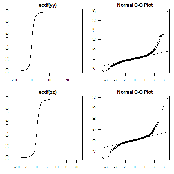
yy <- rLambertW(n=1000, distname="t", theta = theta.st)

# double heavy-tail Lambert W x Gaussian (= Tukey's hh)
zz =<- rLambertW(n=1000, distname = "normal", theta = theta.hh)

### Plot ecdf and qq-plot ####
op <- par(no.readonly=TRUE)
par(mfrow=c(2,2), mar=c(3,3,2,1))
plot(ecdf(yy))
qqnorm(yy); qqline(yy)

plot(ecdf(zz))
qqnorm(zz); qqline(zz)
par(op)

In practice, of course, you have to estimate $\theta = (\beta, \delta)$, where $\beta$ is the parameter of your input distribution (e.g., $\beta = (\mu, \sigma)$ for a Gaussian, or $\beta = (c, s, \nu)$ for a $t$ distribution; see paper for details):

### Parameter estimation ####
mod.Lst <- MLE_LambertW(yy, distname="t", type="s")
mod.Lhh <- MLE_LambertW(zz, distname="normal", type="hh")

layout(matrix(1:2, ncol = 2))
plot(mod.Lst)
plot(mod.Lhh)

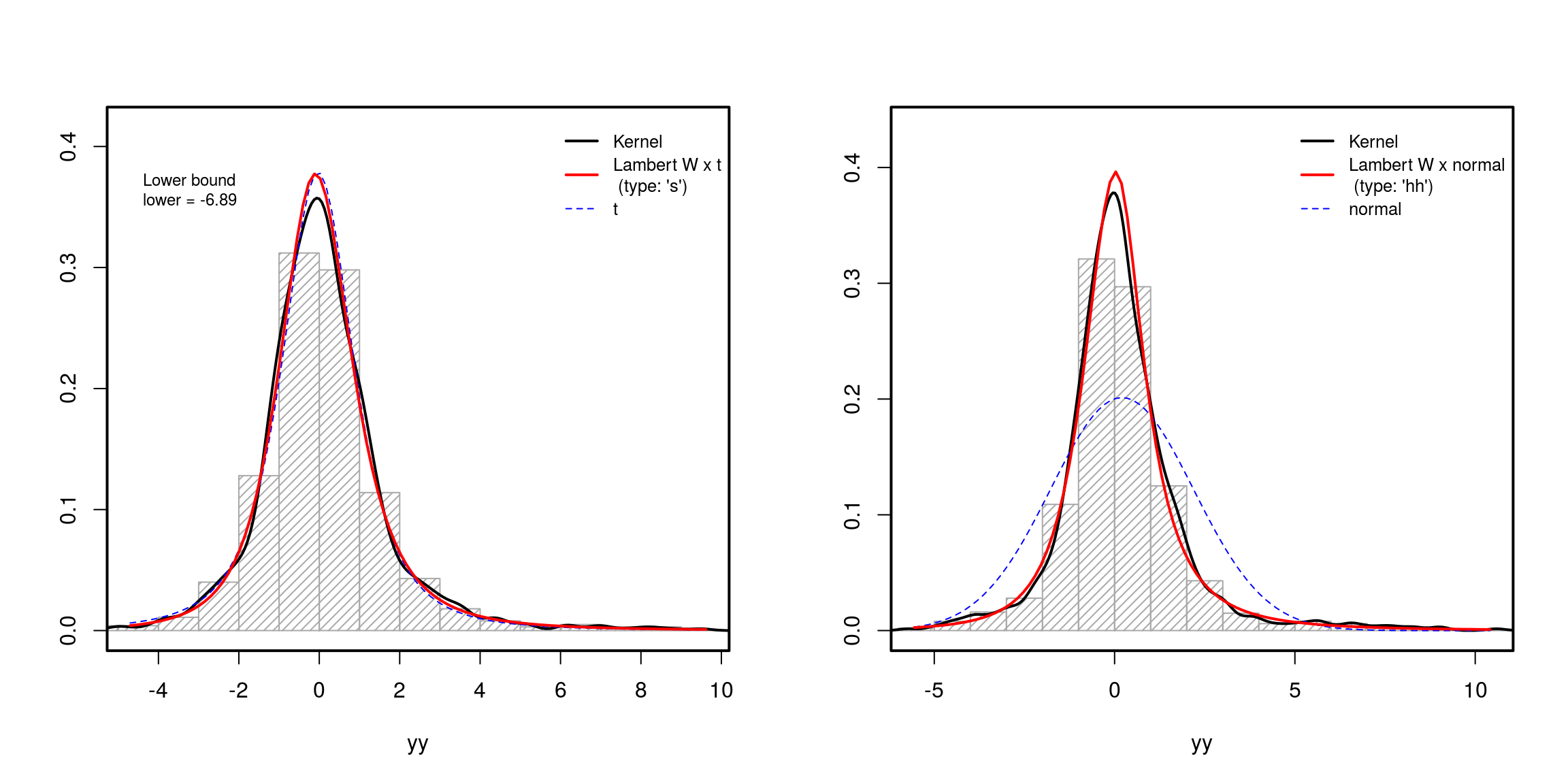
Since this heavy-tail generation is based on a bijective transformations of RVs/data, you can remove heavy-tails from data and check if they are nice now, i.e., if they are Gaussian (and test it using Normality tests).

### Test goodness of fit ####
## test if 'symmetrized' data follows a Gaussian
xx <- get_input(mod.Lhh)
normfit(xx)

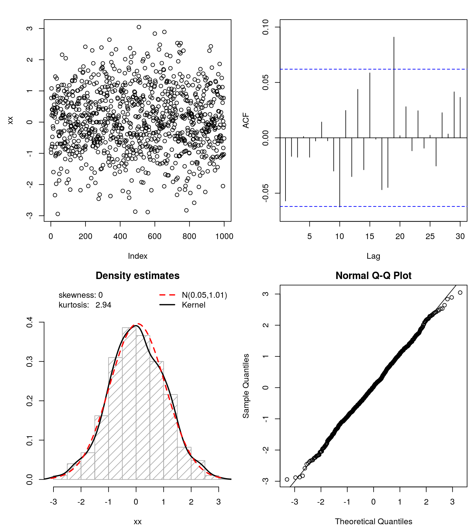
This worked pretty well for the simulated dataset. I suggest you give it a try and see if you can also Gaussianize() your data.

However, as @whuber pointed out, bimodality can be an issue here. So maybe you want to check in the transformed data (without the heavy-tails) what's going on with this bimodality and thus give you insights on how to model your (original) data.

Answer 2

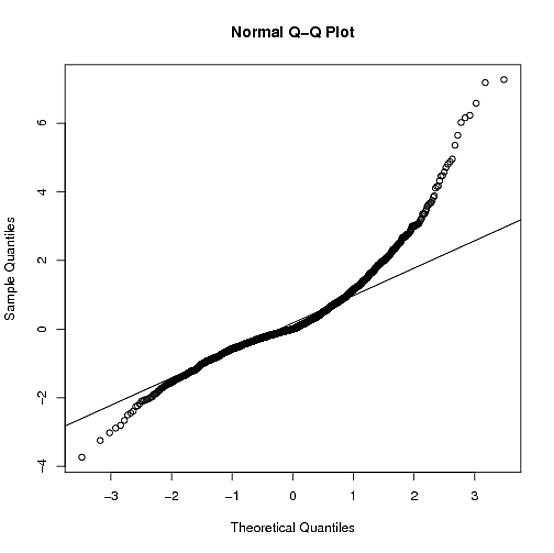
This looks like an asymmetric distribution that has longer tails, in both directions, than the normal distribution.

• You can see the long-tailedness because the observed points are more extreme than those expected under the normal distribution, on both the left and right side (i.e. they are below and above the line, respectively).

• You can see the asymmetry because, in the right tail, the extent to which the points are more extreme than what would be expected under normal distribution is greater than it is in the left tail.

I can't think of any "canned" distributions that have this shape but it's not too hard to "cook up" a distribution that has the properties stated above.

Here is a simulated example (in R):

set.seed(1234)
x=rexp(1e3)
y=-rexp(1e3,rate=2)
z=c(x,y)
qqnorm(z)
qqline(z) # see below for the plot. 
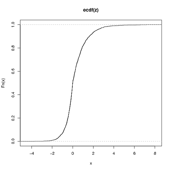
plot( ecdf(z) ) # see below for plot (2nd plot)

The variable here is a 50/50 mixture between an ${\rm exponential}(1)$ and an ${\rm exponential}(2)$ reflected around 0. This choice was made because it will be definitionally asymmetric, since there are different rate parameters, and they will both be long-tailed relative to the normal distribution, with the right tail being longer, since the rate on the right hand side is larger.

This example produces a pretty similar qqplot and empirical CDF (qualitatively) to what you're seeing:

Answer 3

In order to figure which distribution is the best fit, I would first identify some potential target distributions: I would think about the real world process that generated the data, then I would fit some potential densities to the data and compare their loglikelihood scores to see which potential distribution fit best. This is easy in R with the fitdistr function in the MASS library.

If your data is like Macro's z then:

>fitdistr(z,'cauchy',list(location=mean(z),scale=sqrt(sd(z))))$loglik
[1] -2949.068

> fitdistr(z,'normal')$loglik
[1] -3026.648

> fitdistr(z,'t')$loglik
[1] -2830.861

So this gives the t distribution as best fitting (of those we tried) for Macro's data. confirm this with some qqplots using the parameters from fitdistr.

> qqplot(z,rt(length(z),df=2.7))  

Then compare this plot to the other distribution fits.