Grid based piecewise-stationary Poisson process test

Question

I'm trying to fit a set of data to a variety of Poisson-based models, and have hit a stumbling block when trying to fit a piecewise-stationary Poisson process. What I mean by this is a Poisson process that has intensity $\lambda_1$ for time interval $T_1$, then intensity $\lambda_2$ for the time interval $T_2 = T - T_1$, where $T$ is the total observational period.

The likelihood function that I'm using for observing $N_1$ events in that first time interval and $N_2$ events in the second is:

$${Pr(N_1, N_2 | \lambda_1, \lambda_2, \Delta T_1)} = \frac{\left(\lambda_1 \Delta T_1\right)^{N_1} \textit{e}^{-\lambda_1 \Delta T_1}}{N_1 !} \frac{\left(\lambda_2 (T-\Delta T_1\right))^{N_2} \textit{e}^{-\lambda_2 (T-\Delta T_1)}}{N_2 !}$$

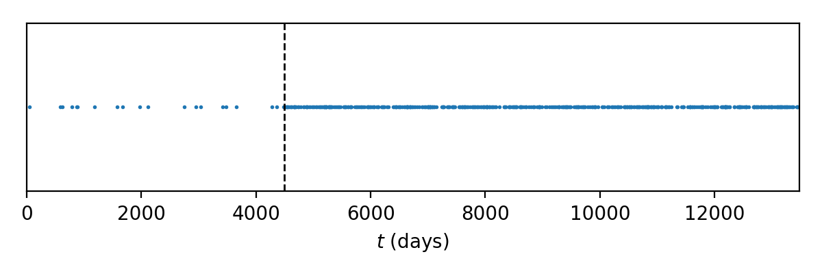
For testing purposes I create a set of fake data that should have a very clear signal of a rate change by generating 20 events uniformly distributed within the interval $t=0$ and $t=4500$, then 500 events uniformly distributed within the interval $t=4500$ and $t=13500$. An example of this is below.

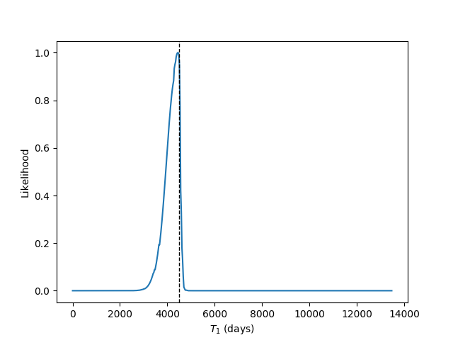
If I fix the two intensities, $\lambda_1$ and $\lambda_2$, to be constant, and equal to their expected value based on the model (0.00445, 0.0556 respectively), then scan through various choices of $T_1$ we can see the one dimensional likelihood as a function of $T_1$ below. It shows that (as expected) the most likely hypothesis is one with $T_1 \sim 4500$ (dashed black line indicates the true simulation parameter).

I then generate a 500x500x500 3D grid of likelihoods, spanning uniform ranges of $\lambda_1$, $\lambda_2$, and $T_1$, noting that $N_1$ and $N_2$ vary as a function of $T_1$. When I marginalise this probability grid over different combinations of parameters things start to not make sense to me any more. In doing this marginalisation I adopt bounded uniform priors on all three parameters (janky looking start/end points chosen to avoid some computational problems at boundaries of the grid): $$\lambda_1 \sim \text{Unif}(1\times10^{-4},\ 1.36\times10^{-2})$$ $$\lambda_2 \sim \text{Unif}(1\times10^{-4},\ 1.67\times10^{-1})$$ $$T_1 \sim \text{Unif}(1,\ 13499)$$

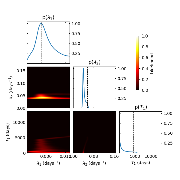
By marginalising over any two of the parameters, I should find the posterior distribution for the third parameter (up to a constant normalisation factor thanks to the uniform priors). I plot all of these, plus the 2D marginalised likelihood surfaces for all combinations of parameters below.

It is self-consistent: the 2D plots, when integrated along either axis give you the 1D posteriors. The black dashed lines show the true simulation parameters for $\lambda_1$, $\lambda_2$, $T_1$. It's clear that the posteriors for $\lambda_2$ and $T_1$ do not adequately include the true simulation parameter.

I'm not sure what's going wrong! The more events I test with the more extreme (sharp) the posteriors become, while getting no closer to the simulation parameter they should be estimating.

I then tried to visualise the likelihoods on a 3d grid (see the gif linked here, each point in the grid is coloured and transparencied in proportion to the likelihood at that point, yellow/solid being most likely while purple/faint being least likely) it's clear that the maximum likelihood points do lie on the $T_1=0$ plane. There is a very slight local maximum away from the boundaries of the likelihood grid (hard to see in the gif due to the coarseness of that grid), at the true simulation parameters, but it is 10 times less likely than the points on the edge, and it drops off fairly fast in any direction away from that local maximum.

---

Is this grid based method just the wrong way to go about this kind of test? Am I doing/missing something obvious/silly? Are the uniform priors causing problems? Do I have to move to a MCMC/other method for finding posteriors?

Answer 1

You have made a slight, but important, mistake in your likelihood function. Let's try constructing it differently, breaking the $T=13,500$-length time period into $13,500$ time periods of length $1$ instead of two time periods of length $T_1$ and $T-T_1$. You can see how that likelihood function will look:

$$\mathcal{L}(\lambda_1, \lambda_2, T_1) = {\lambda_1^{N_1} e^{-\lambda_1 T_1} \over \Pi_{t\leq T_1}x_t!}{\lambda_2^{N_2} e^{-\lambda_2 (T-T_1)} \over \Pi_{T_1 <t\leq T}x_t!}$$

where $\lambda_1$ is the per-period arrival rate in $[0,T_1]$, $x_t$ is the total number of arrivals in period $t$, $N_1$ is the total number of arrivals in $[0,T_1]$, etc.

The way you have done it implicitly assumes there are two periods, one with rate $\lambda_1T_1$ and one with rate $\lambda_2 (T-T_1)$, but if you examine those expressions carefully, you will see that you are confounding the arrival rates $\lambda_i$ and $T$; you really only have two arrival rates in your likelihood function, rates which are functions of the three parameters $\lambda_1$, $\lambda_2$, and $T$, and two samples, each of size $1$.

To see this more clearly, let's rewrite your version of the probability distribution of the data:

$$p(N_1,N_2) = {\gamma_1^{N_1}e^{-\gamma_1} \over N_1!}{\gamma_2^{N_2}e^{-\gamma_2} \over N_2!}$$

where $\gamma_1 = \lambda_1\Delta T_1$ and $\gamma_2 = \lambda_2(T-\Delta T_1)$. The first term is the probability of a single observation $N_1$ from a Poisson($\gamma_1$), and the second is the probability of a single observation $N_2$ from a Poisson($\gamma_2$). We can learn about $\gamma_1$ and $\gamma_2$, but not so much about $\lambda_1$, $\lambda_2$, and $T_1$. For example, if the MLEs of $\gamma_1$ and $\gamma_2$ are 1 and 2 respectively, with the maximum likelihood function value $\mathcal{L}(1,2) = 1$, then setting $T=10$, $T_1=5$, $\hat{\lambda}_1 = 0.2$, and $\hat{\lambda}_2 = 0.4$ results in $\mathcal{L}(0.2*5=1, 0.4*5=2) = 1$, and setting $T_1 = 2$, $\hat{\lambda}_1 = 0.5$, and $\hat{\lambda}_2 = 0.25$, results in $\mathcal{L}(0.5*2=1, 0.25*8=2) = 1$, the same as before. Any value of $T_1$ has corresponding values of $\hat{\lambda}_1$ and $\hat{\lambda}_2$ that allow the maximum of the likelihood function to be achieved, so all values of $T_1$ are equally likely and the likelihood function contains no information about $T_1$. (It does contain information about the relationship between $T_1$, $\lambda_1$, and $\lambda_2$, but not about $T_1$ in isolation.)

This way makes $T_1$ and $T-T_1$ into two sample sizes, and thereby separates them from the arrival rates per observation. We still have $\lambda_1T_1$ and $\lambda_2(T-T_1)$ in the exponential term because there are $T_1$ periods; taking the product of $T_1$ Poisson distributions results in a term of the form $\exp\{-\lambda T_1\}$ (and, in this case, $\exp\{-\lambda(T-T_1)\}$).

On a more intuitive level, by treating each $x_t$ as a sample, we can distinguish between the following two situations. Let $T_1 = 9,000$ and $N_1 = 320$. Now, if there were 20 observations over the first 4500 periods and 300 over the last 4500 periods, that would be extraordinarily unlikely for a Poisson variate, and would weigh very heavily against the hypothesis of a constant rate over the interval, but if there were 155 observations over the first 4500 periods and 165 over the last 4500 periods, that wouldn't be unusual at all. However, if we aggregate all the counts to $N_1 = 320$, we can't distinguish between these two arrangements of the observations, even though all the information is there in the underlying data. It is this information that is being lost by your aggregation of the data into one observation from each of two time periods.

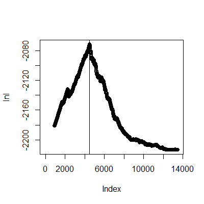
We'll show some R code that calculates the profile log likelihood for $T_1$, that is, the log likelihood for $T_1$ given the maximum likelihood estimators for $\lambda_1$ and $\lambda_2$ conditional upon $T_1$.

time_stamps <- sort(c(4500*runif(20), 
                      4500+9000*runif(500)))

ln_l <- function(T) {
   N1 <- sum(time_stamps <= T)
   N2 <- sum(time_stamps > T)

   l1 <- N1 / T
   l2 <- N2 / (13500-T)

   list(lambda_hat_1 = l1,
        lambda_hat_2 = l2,
        lnl = N1*log(l1) + N2*log(l2) - l1*T - l2*(13500-T))
}

lnl <- rep(0, 13500)
for (i in seq_len(length(lnl))) {
   lnl[i] <- ln_l(i)$lnl
}

plot(lnl)
abline(v=4500)

which.max(lnl)  # The MLE of T1
[1] 4491

ln_l(which.max(lnl)) $ The MLEs of lambda_1, lambda_2
$lambda_hat_1
[1] 0.004230684

$lambda_hat_2
[1] 0.05561106

$lnl
[1] -2071.418

The resulting plot looks like:

You can avoid the discretization into $13,500$ periods by converting the problem to one of estimating the parameters of the two exponential distributions for the inter-arrival times, but you would gain very, very little for a problem of this size by doing so.

ETA: Some question has arisen as to why the above code omits the factorials in the denominator. This is because they are functions only of the $x_i$, and, as such, don't change when the input values to the likelihood function change; they are constants, and can be ignored.

Consider the log of the likelihood function for a Poisson (which saves me typing relative to the actual problem):

$$\log \mathcal{L}(\lambda) = -N\lambda + \log(\lambda)\sum x_i - \sum \log x_i!$$

Let's take the difference for two values of $\lambda$, an operation which occurs inside the deviance / AIC / BIC calculations:

$$\log \mathcal{L}(\lambda_1) - \log \mathcal{L}(\lambda_2) = -N(\lambda_1-\lambda_2) + (\log(\lambda_1)-\log(\lambda_2))\sum x_i$$

as the two terms involving $\sum \log x_1!$ cancel out. It should also be clear that the maximum value of $\log \mathcal{L}(\lambda)$ will be achieved at the same value of $\lambda$ regardless of whether the additive term $\sum \log x_i!$ is included or not, and all the slopes and higher level derivatives will also be the same. Thus, performing the calculations with $x!$ adds nothing to our analysis except computational burden.

From a Bayesian point of view, consider the following posterior distribution:

$$f(\lambda;x) = C{\lambda^xe^{-\lambda} \over x!}p(\lambda)$$

where $p(\lambda)$ is the prior on $\lambda$ and $C$ is the unknown constant of integration required to make $f$ integrate to 1. Let's calculate $C$:

$$C = {1 \over {1 \over x!}\int_0^{\infty}\lambda^xe^{-\lambda}p(\lambda)d\lambda} = C'x!$$

Replacing $C$ with $C'x!$ results in:

$$f(\lambda;x) = C'\lambda^xe^{-\lambda}p(\lambda)$$

as the terms involving $x!$ cancel out. Note that $C'$ does not change if we leave $1/x!$ out of the denominator of the expression for $C$. This shows that we don't need to include the $x!$ in the first place; it will just be canceled out when calculating the constant of integration anyway, so it adds no value.