How to calculate the confidence that a trend in a time-series is positive?

Question

Every year a random population sample of 10,000 people is asked whether they like apples. The results are:

Year    % likes apples
2013    4.4%
2014    4.1%
2015    5.5%
2016    6.3%
2017    5.4%
2018    6.0%

Standard deviation = 0.87%

Using the data, I want to be able to say:

• We can be X% confident that the percentage of people who like apples increased between 2013 and 2018.
• We can be 95% confident that the percentage of people who like apples increased by at least Y% between 2013 and 2018.

But I don’t know how to calculate the values for X and Y.

I’m quite confused about this. Linear trend estimation seems to be the relevant concept here but I haven’t managed to understood how to apply it.

Answer 1

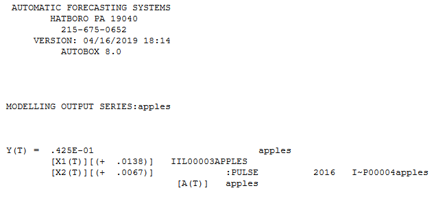
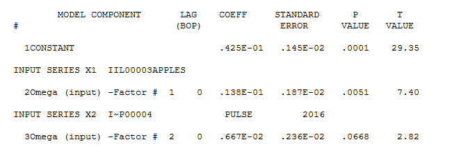
The data you describe is what might be considered summary statistics. Whether somebody likes apples can be considered a binary outcome (1 = likes apples, 0 = doesn't like apples). Therefore, if you survey 10,000 people over 6 years then you have 60,000 responses measuring the binary outcome of whether each individual likes apples.

The probability that somebody likes apples is actually the mean value of the binomial outcome. This is important for two primary reasons:

1. The sample size is much larger than summary statistics you have presented, and therefore you should have much higher confidence in your results than linear regression of summary statistics would indicate

2. The binary nature of your data should lead you to consider logistic regression.

I don't have the complete data since you only provided summary statistics. To illustrate the approach I will simulate some data assuming your probabilities of liking apples are in fact the "true" probabilities.

library(dplyr)
library(ggplot2)
library(tidyr)


# Simulate some data ------------------------------------------------------

# Number of individuals
n.individuals <- 1e4

# Years of study
years <- 2013:2018

# Numbre of years
n.years <- length(years)

# Probability of liking apples 
pLikeApples = c(0.044, 0.041, 0.055, 0.063, 0.054, 0.060)

# Matrix of data
# Rows = individuals
# Columns = years
likesApples <- matrix(rep(NA_integer_, n.individuals*n.years), nrow = n.individuals)
for (j in 1:n.years) {
  for (i in 1:n.individuals) {
    likesApples[i,j] <- rbinom(1, 1, pLikeApples[j])
  }
}

# Name columns
colnames(likesApples) <- years

# Convert to data frame
appleData <- as_tibble(likesApples) %>% 
  mutate(ID = row_number()) %>% 
  gather(year, likesApples, -ID) %>% 
  mutate(year = as.integer(year))

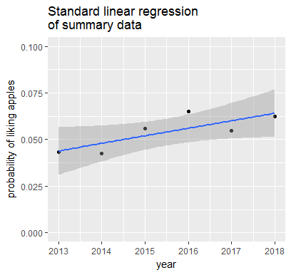
If we perform simple linear regression on summary statistics then we obtain results as shown below

# Summary data ------------------------------------------------------------

summaryAppleData <- 
  appleData %>% 
  group_by(year) %>% 
  summarize(pLikeApples = mean(likesApples))

# Plot data ---------------------------------------------------------------

ggplot(summaryAppleData,
       aes(x = year, y = pLikeApples)) +
  geom_point() +
  geom_smooth(method = "lm") +
  labs(title = "Standard linear regression \nof summary data",
       y = "probability of liking apples") +
  ylim(0, 0.1)

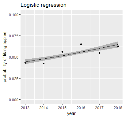
If we use the complete data and apply logistic regression then we obtain results as shown below

# Logistic regression -----------------------------------------------------

# Fit logistic regression model
myMod <- glm(data = appleData,
             formula = likesApples ~ year,
             family = "binomial")

# Summarize model
summary(myMod)

# Inverse link function
linkInv <- myMod$family$linkinv

# Predict response on linear scale
predLink <- predict.glm(myMod, newdata = summaryAppleData, type = "link", se.fit = TRUE)

# Backtransform predictions
pred <- 
  summaryAppleData %>% 
  mutate(pred = linkInv(predLink$fit),
         LL = linkInv(predLink$fit - 1.96*predLink$se.fit),
         UU = linkInv(predLink$fit + 1.96*predLink$se.fit))

# Plot logistic regression
ggplot() +
  geom_point(data = summaryAppleData, aes(x = year, y = pLikeApples)) +
  geom_line(data = pred, aes(x = year, y = pred)) +
  geom_ribbon(data = pred, aes(x = year, y = pred, ymin = LL, ymax = UU), alpha = 0.3) +
  labs(title = "Logistic regression",
       y = "probability of liking apples") +
  ylim(0, 0.1)

Finally to address your first question, based on the summary of the logistic regression model we see that the year variable is significant with a significant code of *** indicating a confidence level of basically 100%. You need to run the analysis on your data and not simulated data as I have done. Also, as discussed by @orcmor you should use caution when interpreting the confidence level. However, this indicates a significant increase in the probability of liking apples over time.

Your second question is slightly more complicated. You are interested in how much the response Y has changed for a range of X values. A ballpark estimate might be to take the upper end of the 95% confidence interval for the mean probability in 2013 and take the lower end of the confidence interval for 2018 to get an approximate lower bound on the total change. From the data I simulated, this is about a 1.4 percentage point increase.

Answer 2

I suggest you take a quick look at hypothesis testing concepts if you already had not done it for understanding what is meant by confidence. In hypothesis testing, you make the distinction that your observed sample is a realization of your data generating process and is susceptible to random deviations from the exact function. Consequently, your estimation of the coefficients could be off due to random errors as well. Confidence, in this context, usually refers to the unlikeliness of your sample being deviated by random errors. You basically want to say that, given this sample, there is a X% chance that I did not observe this sample (and my conclusions) by random error. In order to be able to say this, you have to make an assumption on the distribution of errors so that you can calculate the distribution of your estimations.

If your function is:

$$ appleLiking = \beta_0 + \beta_1 t + \epsilon $$

then you can answer both of your question if you know the mean and variance of your $\beta_1$ estimation.

• For your first question, you are interested in how close your estimated $\hat\beta_1$ is to $0$, given your estimated $\hat\beta_1$ variance. This is commonly referred as the significance of $\hat\beta_1$.

• For your second one, you are interested in how close your estimated $\hat\beta_1$ is to $Y$, given your estimated $\hat\beta_1$ variance.

Luckily, once you assume the distributions, the estimations are relatively straightforward statistical procedures. You calculate the confidence levels by common p-values using standard normal distributions. For the estimation procedure, since you are asking a time-series, you may go with ARIMA estimations to account for autocorrelations in error term. If you are using R, the following will provide an estimation:

appleLiking = as.ts(c(0.044, 0.041, 0.055, 0.063, 0.054, 0.060))    
auto.arima(appleLiking, xreg=1:length(appleLiking))

Notice the standard errors displayed. Those values are the ones you need for confidence calculations. See the answers here for more details on time series issues.

Answer 3

A more data-driven analysis i.e. less presumptive of the form of the model... detecting the presence of a level shift and NO TREND ... this uses 3 parameters rather than two which was used in the simple and presumptive trend model in time.

leading to the detection of a pulse at 2016

enter image description here

In summary building and identifying a model with 6 observations is tough at best .. The whole idea is to form a model that is more representative of the data.

You asked "can be X% confident that the percentage of people who like apples increased between 2013 and 2018." .. the answer is yes with 99.49 % confidence .