Getting 1-tailed p value from a 2-tailed p value in SPSS v23

Question

For the purpose of my research, I use IBM SPSS and would like to get paired t-test result with a 1-tailed p-value.

This video states how to derive a 1-tailed p-value from 2-tailed p-value, however, me and my mentor aren't sure of such a way would produce an accurate result.

https://youtu.be/UaGMEPaSaFo?t=156

If you need more information - let me know and I will update the question.

Edit 1 As I read form comments, it is an appropriate way to do it, and I update the question to be less dependant on the video.

All I wanted to ensure is how to get 1-tailed p-value both ways from a 2-tailed p-value and verify if the following ways are scientifically and statistically accurate for a master degree thesis.

Left-tailed = p/2

Right-tailed = 1 - (p/2)

(cited from sparc_spread here: Doubling &/or halving p-values for one- vs. two-tailed tests)

Let me know how I can improve this question/answer. Thank you again.

Answer 1

Just to be sure you understand the relationship between one- and two-sided P-values for a one-sample t test, here are some examples.

First, some fake data to use for illustration. [Use the same set.seed statement to get exactly the same data I use here; omit set.seed or pick a different seed for fresh data.]

set.seed(729); x = rnorm(16, 115, 20)
mean(x);  sd(x)
[1] 111.9711    # sample mean
[1] 24.54165    # sample SD

Two-sided test: Use the t.test procedure in R to test $H_0: \mu = 100$ against the 2-sided alternative $H_a: \mu \ne 100.$ [A 2-sided alternative is the default.] The P-value is about $0.07 > 0.05,$ so we do not reject $H_0.$

t.test(x, mu = 100)

        One Sample t-test

data:  x
t = 1.9512, df = 15, p-value = 0.06997
alternative hypothesis: true mean is not equal to 100
95 percent confidence interval:
  98.89381 125.04846
sample estimates:
mean of x 
 111.9711 

The P-value is computed as follows: Under $H_0,$ the test statistic $T = \frac{\bar X - 100}{S/\sqrt{16}} \sim \mathsf{T}(15).$ The P-value is computed as $P(|T| \ge 1.9512) = 2P(T \ge 1.9512) = 2(1 - P(T \le 1.9612)) = 0.06997 \approx 0.07.$

2*(1 - pt(1.9512, 15))
[1] 0.0699666

Right-sided test: Use the t.test procedure in R to test $H_0: \mu = 100$ against the right-sided alternative $H_a: \mu > 100.$ [Note the parameter alt="gr".] The P-value is about $0.035 < 0.05,$ so we reject $H_0.$

t.test(x, mu = 100, alte="gr")

        One Sample t-test

data:  x
t = 1.9512, df = 15, p-value = 0.03499
alternative hypothesis: true mean is greater than 100
95 percent confidence interval:
 101.2154      Inf
sample estimates:
mean of x 
 111.9711 

Notice that one could cheat by 'deciding', after a look at results of the two-sided test, that the a one-sided test "Was really intended all along." to get the smaller P-value and the resulting smaller P-value, permitting rejection. That is why it is good practice to state, in advance of seeing the data, whether a one-tailed or two-tailed test will be performed.

The P-value is computed as follows: Under $H_0,$ the test statistic $T = \frac{\bar X - 100}{S/\sqrt{16}} \sim \mathsf{T}(15).$ Then $P(T \ge 1.9512) = P(T \ge 1.9512) = 1 - P(T \le 1.9612) = 0.06997 \approx 0.035.$

1 - pt(1.9512, 15)
[1] 0.0349833

Left-sided test: Use the t.test procedure in R to test $H_0: \mu = 100$ against the left-sided alternative $H_a: \mu < 100.$ [Note the parameter alt="less".] The P-value is about $0.965 >> 0.05,$ so we do not reject $H_0.$

t.test(x, mu = 100, alte="less")

        One Sample t-test

data:  x
t = 1.9512, df = 15, p-value = 0.965
alternative hypothesis: true mean is less than 100
95 percent confidence interval:
     -Inf 122.7268
sample estimates:
mean of x 
 111.9711 

Of course, one rejects $H_0$ when the P-value is very small. However, when the P-value is very near $1,$ that may be an indication that something is wrong: it might be wrong type of test for the type of data, incorrect syntax using software, mistake in hand computation, and so on. Here the mistake is that we guessed wrong about the direction of the possible difference from $\mu_0 = 100.$ The sample mean $\bar X > 100$ cannot provide evidence that $H_a: \mu < 100$ could be true.

The P-value is computed as follows: Under $H_0,$ the test statistic $T = \frac{\bar X - 100}{S/\sqrt{16}} \sim \mathsf{T}(15).$ [The P-value is the probability of a more extreme result in the direction of the alternative.)] Then $P(T \le 1.9512) = P(T \ge 1.9512) \approx 0.965.$

pt(1.9512, 15)
[1] 0.9650167

In summary: With enough information we can convert a two-sided P-value into a one-sided P-value. The important information is not whether the alternative is left- or right-sided. It is whether the sample mean $\bar X$ is above or below the hypothetical population mean $\mu_0.$ (Equivalently, whether the test statistic $T$ is positive or negative.

However, in a properly conducted analysis, I don't see why there should ever be a need to do this conversion. One should decide before seeing the data whether the alternative is to be two-sided, left-sided, or right-sided, and compute the test statistic and P-value accordingly.

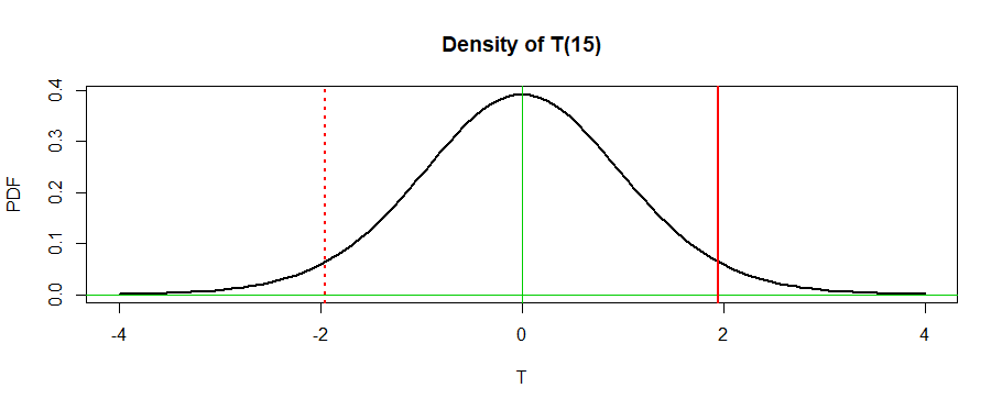
The figure below shows the density function of $\mathsf{T}(15)$ and the value $T = 1.9512$ of the test statistic as a solid vertical line. The P-value of a right-tailed test is the area under the curve to the right of the solid line; the P-value of a two-tailed test is double that area, and the P-value of a left-tailed test is the area under the curve to the left of the solid line.