3
$\begingroup$

I have this data:

Group Time  Size
A 1 0.56
A 2 0.97
A 3 1.33
A 4 1.75
B 1 0.12
B 2 0.24
B 3 0.31
B 4 0.47
B 5 0.51
B 6 0.69
B 7 0.73
B 8 0.85
C 1 0.16
C 2 0.23
C 3 0.38
C 4 0.49
C 5 0.53
C 6 0.66
C 7 0.78
C 8 0.81

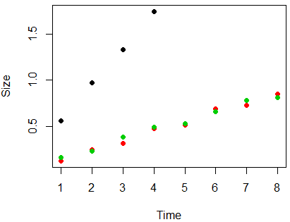
Here is the respective plot:

enter image description here

Now I would like to test the three groups for differences in slope and intercept. I cannot use simple linear regression since these are time series and the data points are not independent of each other.

Here are the additional tests I performed on the linar model:

Data = read.table(textConnection(Input),header=TRUE)

model = lm(Size ~ Time + Group,data = Data)

Shapiro-Wilk test for normality:

shapiro.test(residuals(model))

p=0.001288 (not normally distributed)

Breusch-Pagan test for equal variances:

bptest(model)

p=0.016 (variances not equal)

Since residuals are not normally distributed and variances are not equal an ANOVA (for example) could not be performed. Furthermore, the residuals are auto-correlated according to the Durbin-Watson test:

dwtest(model)

p=0.001065 (data points auto-correlated)

Which model would be suitable for my problem (probably a multilevel linear model?) and which R packages I could use for the analysis?

Another data set:

Input = ("
Group   Time    Size
A   1   1.08152
A   2   1.10589
A   3   1.13292
B   1   1.04597
B   2   1.05763
B   3   1.07023
B   4   1.08612
B   5   1.10059
B   6   1.11589
B   7   1.13143
B   8   1.14741
B   9   1.16721
B   10  1.18288
C   1   1.04777
C   2   1.06145
C   3   1.07484
C   4   1.08908
C   5   1.10346
C   6   1.11866
C   7   1.13375
C   8   1.14931
C   9   1.16563
C   10  1.18294
")
dat = read.table(textConnection(Input),header=TRUE)
$\endgroup$
8
  • 5
    $\begingroup$ Can you elaborate on why you can't use linear regression? Have you tested if residuals are auto-correlated? $\endgroup$
    – Roland
    Commented May 3, 2019 at 12:22
  • $\begingroup$ Yes, I have. I have constructed this model: model = lm(Size ~ Time + Group + Time:Group,data = Data) (according to rcompanion.org/rcompanion/e_04.html) and performed a Durbin-Watson test with dwtest(model). The resulting p-value is 0.002353. Furthermore the data is not normally distributed: shapiro.test(residuals(model)) gives p=0.00795. I hope I did everything right. $\endgroup$
    – Kardashev3
    Commented May 3, 2019 at 12:36
  • 2
    $\begingroup$ Without see your acutal data frame, your model maybe assuming "Group" as a continuous variable and not a categorical value. If you convert "Group" from numeric to a factor and then run the linear regression. The residual plot is more normal and thus a standard linear regression analysis is a safer assumption. Also repeat the analysis without the group/time interaction term. $\endgroup$
    – Dave2e
    Commented May 3, 2019 at 13:34
  • 2
    $\begingroup$ The heteroscedasticity likely derives from the black points, which so obviously have a different slope there is no need to test them. Consider, then, removing those points from the data and focusing on the remaining data. Plotting the linear regression residuals against time would provide useful information about the nature and size of any remaining autocorrelation. $\endgroup$
    – whuber
    Commented May 3, 2019 at 14:22
  • 2
    $\begingroup$ I wasn't suggesting ignoring the black points: my suggestion was to analyze the data as two separate groups. At that point you will have the quantitative backup needed to state the obvious: namely, you will have independent estimates of slopes and the standard errors of estimate. $\endgroup$
    – whuber
    Commented May 6, 2019 at 14:10

4 Answers 4

8
+50
$\begingroup$

This is a relatively simple problem. The basic model to test your question about differences in slope is:

(m0 <- lm(Size ~ Time * Group, dat))
# Coefficients:
# (Intercept)         Time       GroupB       GroupC  Time:GroupB  Time:GroupC  
#      0.1700       0.3930      -0.1482      -0.1032      -0.2890      -0.2956  

I have ignored the question about the intercepts. More on this at the end. Also, the basic model you ran does not permit testing of differences in slopes. If you perform the diagnostic tests you performed on the model m0 here, they do not confirm misspecification.

However, it appears Group A is on a different scale, so it makes sense to run a heteroskedastic model. Additionally, as @whuber pointed out in the comments, it makes sense to model the autocorrelation. I use the simple autocorrelation of order 1:

library(nlme)
(m1 <- gls(Size ~ Time * Group, dat, correlation = corAR1(form = ~ Time | Group),
           weights = varIdent(form = ~ 1 | I(Group == "A"))))
# Coefficients:
# (Intercept)        Time      GroupB      GroupC Time:GroupB Time:GroupC 
#   0.1768985   0.3900313  -0.1543012  -0.1146352  -0.2860587  -0.2912242 
# 
# Correlation Structure: AR(1)
#  Formula: ~Time | Group 
#  Parameter estimate(s):
#        Phi 
# -0.5295663 
# Variance function:
#  Structure: Different standard deviations per stratum
#  Formula: ~1 | I(Group == "A") 
#  Parameter estimates:
#     TRUE    FALSE 
# 1.000000 2.152732 

We find that the residual standard deviations of the groups that are not group A are about double the residual standard deviation for group A. And that there is negative autocorrelation - positive-negative residual switching pattern by time.

To address your primary research questions, we can go:

library(emmeans)
pairs(emtrends(m1, ~ Group, var = "Time"))
#  contrast    estimate          SE df t.ratio p.value
#  A - B    0.286058700 0.005098842 14  56.103  <.0001
#  A - C    0.291224187 0.005098842 14  57.116  <.0001
#  B - C    0.005165488 0.003857697 14   1.339  0.3979
# 
# P value adjustment: tukey method for comparing a family of 3 estimates 

We find that there is not much statistical evidence to conclude that the slopes for Group B and C are different from each other. While there is the evidence to differentiate A from B, and A from C.

Since we have an interaction, it is difficult to consider differences in the intercept. Given the current analysis, the intercept relates to group differences at Time 0 which does not exist in the data, minimum Time is 1. The emmeans package provide an option to view differences between the groups at different values of time:

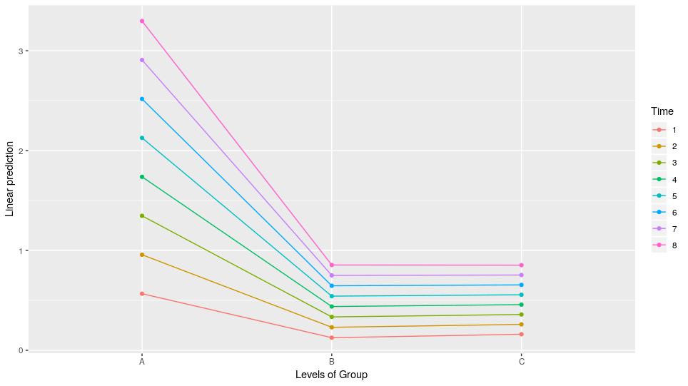
emmip(m1, Time ~ Group, cov.reduce = FALSE)

enter image description here

We find that as time increases, the group differences between A and B, and A and C increase. But B and C continue to be relatively similar. Be careful because there are no time point beyond time 4 for Group A, these are extrapolated values.

Given what we have learned, a parsimonous model would be:

m.pars <- gls(Size ~ Time * I(Group == "A"), dat,
              correlation = corAR1(form = ~ Time | Group),
              weights = varIdent(form = ~ 1 | I(Group == "A")))
$\endgroup$
7
  • 2
    $\begingroup$ +1. It's nice to see how you handle the heteroscedasticity. But, upon rereading the question, I notice it is also concerned about serial correlation over time within each group. This possibility could invalidate most of the testing you have performed throughout the analysis. $\endgroup$
    – whuber
    Commented May 14, 2019 at 17:43
  • 1
    $\begingroup$ @whuber I modified the response to account for the auto-correlation. It did not change much in this application - the patterns in these data are very strong. $\endgroup$ Commented May 14, 2019 at 18:28
  • $\begingroup$ Thank you for this detailed answer! I have indeed used the wrong model, now the tests for the shown data yield respective results. And the slope differences make sense, as you have shown. I have many more data sets with groups that have even less data (only three data pairs, see newly added data above). Here, Shapiro-Wilk test for normality yields p=0.0243 and the result from Durbin-Watson test is highly significant (p<=0.001). $\endgroup$
    – Kardashev3
    Commented May 16, 2019 at 8:14
  • $\begingroup$ With model m1 I see that the residual standard deviations of the groups that are not group A are almost the same as the residual standard deviation for group A. Regarding autocorrelation there is the same residual switching pattern by time. Pair-wise testing using pairs(...) throws an error: „Error in crossprod(x, y) : requires numeric/complex matrix/vector arguments“. I assume that this happens due to the small size of group A? $\endgroup$
    – Kardashev3
    Commented May 16, 2019 at 8:14
  • 1
    $\begingroup$ Pairwise may throw an error because your group variable is string not numeric. I am not sure. If you have many more data sets, can you create a new question to describe why you have many more data sets? Why do you intend to analyze each one separately? $\endgroup$ Commented May 16, 2019 at 13:13
2
$\begingroup$

Because your model uses longitudinal data, it is best to check for the Intraclass Correlation Coefficient (ICC) before assuming independence. However, this particualr model has a small sample size, so it is singular,

require(lme4)
my_lme=lmer(Size~Time+(Time|Group),data=my_data,REML=F)
isSingular(my_lme)
[1] TRUE

Let's try using a Bayesian model with a Wishart variance-covariance prior.

require(blme)
my_blmer=blmer(cov.prior='wishart',fixef.prior=NULL,resid.prior=NULL,
               formula=Size~Time+(Time|Group),data=my_data)
isSingular(my_blmer)
[1] FALSE

So it works now, but make sure you can justify the use of a Wishart prior. Let's check the ICC:

summary(my_blmer)
Cov prior  : Group ~ wishart(df = 4.5, scale = Inf, posterior.scale = cov, common.scale = TRUE)
Prior dev  : -1.4809

Linear mixed model fit by REML ['blmerMod']
Formula: Size ~ Time + (Time | Group)
   Data: my_data

REML criterion at convergence: -7.2

Scaled residuals: 
     Min       1Q   Median       3Q      Max 
-2.74016 -0.23951 -0.04383  0.26814  2.76185 

Random effects:
 Groups   Name        Variance Std.Dev. Corr 
 Group    (Intercept) 0.54671  0.7394        
          Time        0.01784  0.1336   -0.98
 Residual             0.01331  0.1154        
Number of obs: 20, groups:  Group, 3

Fixed effects:
            Estimate Std. Error t value
(Intercept)  0.25213    0.43100   0.585
Time         0.06510    0.07882   0.826

Correlation of Fixed Effects:
     (Intr)
Time -0.970

The ICC is quite large: $0.546/(0.546+0.017+0.133)=0.78$. Thus, you should be using a Hierarchical Linear Model (HLM). Also, because you have a small sample size, you should use a Bayesian HLM.

$\endgroup$
1
  • $\begingroup$ You don't show how OP should check which group time slopes are different from each other. $\endgroup$ Commented May 19, 2019 at 14:29
1
$\begingroup$

Just code your groups as dummy variables, which I think may be what @whuber was suggesting. There is plenty of reference information available on the internet about dummy variables.

Like so:

time <- c(1,2,3,4,1,2,3,4,5,6,7,8,1,2,3,4,5,6,7,8)
size <- c(0.56, 0.97, 1.33, 1.75, 0.12, 0.24, 0.31, 0.47, 0.51, 0.69, 0.73, 0.85, 0.16, 0.23, 0.38, 0.49, 0.53, 0.66, 0.78, 0.81)
groupa <- c(1, 1, 1, 1, 0, 0, 0, 0, 0, 0, 0, 0, 0, 0, 0, 0, 0, 0, 0, 0)
groupb <- c(0, 0, 0, 0, 1, 1, 1, 1, 1, 1, 1, 1, 0, 0, 0, 0, 0, 0, 0, 0)
lm1 <- lm(size~groupa+groupb+time+groupa:time+groupb:time)

> summary(lm1)

Call:
lm(formula = size ~ groupa + groupb + time + groupa:time + groupb:time)

Residuals:
      Min        1Q    Median        3Q       Max 
-0.035833 -0.021012 -0.003583  0.015768  0.043929 

Coefficients:
             Estimate Std. Error t value Pr(>|t|)    
(Intercept)  0.066786   0.022092   3.023  0.00912 ** 
groupa       0.103214   0.041156   2.508  0.02508 *  
groupb      -0.045000   0.031243  -1.440  0.17176    
time         0.097381   0.004375  22.259 2.51e-12 ***
groupa:time  0.295619   0.013413  22.040 2.87e-12 ***
groupb:time  0.006667   0.006187   1.078  0.29946    
---
Signif. codes:  0 ‘***’ 0.001 ‘**’ 0.01 ‘*’ 0.05 ‘.’ 0.1 ‘ ’ 1

Residual standard error: 0.02835 on 14 degrees of freedom
Multiple R-squared:  0.9963,    Adjusted R-squared:  0.9949 
F-statistic: 746.2 on 5 and 14 DF,  p-value: < 2.2e-16

And now your p-value for Shapiro-Wilks is 0.35, for Breusch-Pagan it is 0.45, and for Durbin-Watson it is 0.92.

For group A your equation is size = (0.066786+0.103214)+(0.097381+0.295619)*time.

Except I would probably run it again without 'groupb' and 'groupb:time', to get a single fitted line for groups B+C together.

$\endgroup$
4
  • $\begingroup$ With a longitudinal model, you need to check the ICC as in an HLM. $\endgroup$ Commented May 10, 2019 at 18:37
  • $\begingroup$ @JaySchylerRaadt, thanks for the feedback, but too much jargon! What is 'ICC' and 'HLM'? Please use the unabbreviated terms so I have some chance to look up what you're talking about... $\endgroup$
    – Izy
    Commented May 10, 2019 at 19:27
  • $\begingroup$ Intraclass Correlation Coefficient (ICC) and Hierarchical Linear Model (HLM) $\endgroup$ Commented May 10, 2019 at 20:00
  • $\begingroup$ Thanks. I've suggested adding the full terms in as an edit to your answer. $\endgroup$
    – Izy
    Commented May 10, 2019 at 20:11
1
$\begingroup$

If you're looking to fit a Bayesian MLM in R, look no further than the rethinking package. You also need to install RStan.

library(rethinking)
Input = ("
         Group   Time    Size
         A   1   1.08152
         A   2   1.10589
         A   3   1.13292
         B   1   1.04597
         B   2   1.05763
         B   3   1.07023
         B   4   1.08612
         B   5   1.10059
         B   6   1.11589
         B   7   1.13143
         B   8   1.14741
         B   9   1.16721
         B   10  1.18288
         C   1   1.04777
         C   2   1.06145
         C   3   1.07484
         C   4   1.08908
         C   5   1.10346
         C   6   1.11866
         C   7   1.13375
         C   8   1.14931
         C   9   1.16563
         C   10  1.18294
         ")
dat = read.table(textConnection(Input),header=TRUE)
simplemodel <- map2stan(
  alist(
    Size ~ dnorm( mu , sigma ) , #normally distributed likelihood function
    mu <- a[Group] + b * Time, #varying intercept by variable "Group"
    a[Group] ~ dnorm( a_mu , a_sigma ), #adaptive priors, b/c IDK
    b ~ dnorm(time_mu, time_sigma),
    a_mu ~ dnorm(0,1),
    a_sigma ~ dcauchy(0,2.5),
    time_mu ~ dnorm(0,1),
    time_sigma ~ dcauchy(0,2.5),
    sigma ~ dcauchy(0, 2.5) #prior to sigma
  ),
  data=dat, iter=1000, warmup=100, chains=1, verbose=T, 
  cores=4, control = list(adapt_delta = 0.99, max_treedepth = 15))

From there, use the precis function do get your coefficients.

> precis(simplemodel, depth = 2)
           mean   sd  5.5% 94.5% n_eff Rhat
a[1]       1.08 0.00  1.07  1.08   712 1.00
a[2]       1.03 0.00  1.02  1.03   964 1.00
a[3]       1.03 0.00  1.02  1.03   846 1.00
b          0.02 0.00  0.01  0.02   886 1.00
a_mu       1.03 0.15  0.88  1.17   399 1.00
a_sigma    0.13 0.22  0.02  0.45    88 1.00
time_mu    0.00 0.67 -1.17  1.11   199 1.00
time_sigma 1.60 1.97  0.13  4.52   165 1.01
sigma      0.00 0.00  0.00  0.01   426 1.00
$\endgroup$

Your Answer

By clicking “Post Your Answer”, you agree to our terms of service and acknowledge you have read our privacy policy.

Not the answer you're looking for? Browse other questions tagged or ask your own question.