2
$\begingroup$

Assume an attribute is normally distributed. Assume we sample from the top 5% of that distribution. Assume we measure the attribute with a multiple-choice test. Assume the difficulty level of the m/c test is such that the average difficulty is p=.5

The scores on the m/c test will tend to be normally distributed due to the test score being based on the binomial distribution.

But the underlying attribute is not normally distributed in the population we are sampling from (since the population for the sake of this quesion is the top 5% of a normal distribution).

Will the data reflect the tail of the normal distribution that we are sampling from, or will the data reflect a normal distribution due to the m/c measuring tool?

$\endgroup$
21
  • 2
    $\begingroup$ Re: "The scores on the m/c test will tend to be normally distributed:" be careful here. The scores attained by a given individual, upon independent repetitions of the test, may well be approximated by a Normal distribution provided the test has enough independent questions. But this says nothing at all about how the scores will vary from one individual to another! $\endgroup$
    – whuber
    Commented Jun 3, 2019 at 15:42
  • $\begingroup$ @whuber Do you care to comment on the simulation in BruceET's answer? $\endgroup$
    – Joel W.
    Commented Jun 4, 2019 at 13:22
  • 1
    $\begingroup$ BruceET remarked that his simulation "validat[es] @whuber's cautionary comment." I agree--and you don't need to know R to appreciate its implications: just look at the histogram. One can obtain even more convincing results by recognizing that your question doesn't stipulate that the score on the test is a linear function of the underlying attribute (an assumption unlikely to be true in most applications, anyway). It is therefore possible that the spread in scores among the top 5% could be extremely skewed. $\endgroup$
    – whuber
    Commented Jun 4, 2019 at 13:36
  • 1
    $\begingroup$ For an actual example of that, see the statistics on top-scoring individuals in the annual Putnam competition. $\endgroup$
    – whuber
    Commented Jun 4, 2019 at 13:36
  • 1
    $\begingroup$ @whuber. That brings us back to my question, "Will the data reflect the tail of the normal distribution that we are sampling from, or will the data reflect a normal distribution due to the m/c measuring tool?" I am interested in looking at the underlying distribution the human ability and not be misled by the distribution of the measurement tool. Is there a way to do that? $\endgroup$
    – Joel W.
    Commented Jun 4, 2019 at 15:24

1 Answer 1

3
$\begingroup$

I suppose you intend that those at the upper end of the attribute scale will do better on the exam. One simple and direct way to model this is to take the attribute to be the probability $p$ of success on each of 100 T/F exam questions.

Suppose there are 20,000 potential subjects with $p \sim \mathsf{Norm}(\mu=0.5, \sigma=0.1).$ Then we pick the top 1000 of them (5%). The score of the $i$th participant is taken to be $X_i \sim \mathsf{Binom}(100, p_i),$ for $i = 1, 2, \dots, 1000.$

I have no idea whether this is a realistic model, but it might be a starting point towards clarifying what kind of model you have in mind. [If the attribute is precisely exam-taking ability, a beta distribution for $p$ might be a better choice than normal.]

set.seed(603)
p = sort(rnorm(20000, .5, .1), decr=T)[1:1000]
s = rbinom(1000, 100, p)
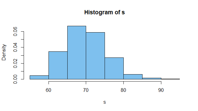
hist(s, prob=T)
summary(s)
   Min. 1st Qu.  Median    Mean 3rd Qu.    Max. 
  56.00   66.00   70.00   70.25   74.00   93.00 

tab = cbind(p,s)
head(tab)
             p  s  # scores of 6 highest 'attribute' subj
[1,] 0.9222469 89
[2,] 0.9020532 90
[3,] 0.8966595 93
[4,] 0.8706467 85
[5,] 0.8425157 85
[6,] 0.8409540 87

tail(tab)
                p  s   
 [995,] 0.6655590 68    # ...and of 6 lowest
 [996,] 0.6655020 67
 [997,] 0.6653522 62
 [998,] 0.6653462 74
 [999,] 0.6652848 74
[1000,] 0.6652532 61

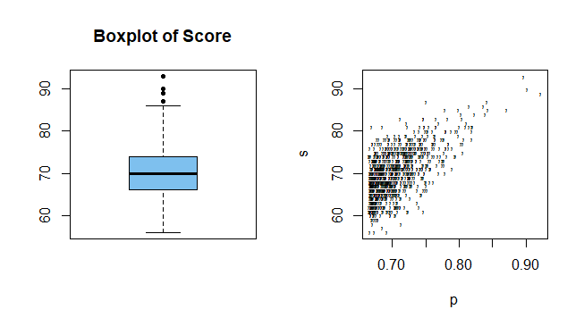
Although the mean and median scores are nearly the same (both around 70), the histogram and the boxplot of the 1000 simulated scores both show some right-skewness--as you anticipated. A Shapiro-Wilk tests rejects the null hypothesis that the scores are normal (validating @whuber's cautionary comment).

 shapiro.test(x)$p.val
 [1] 0.001612833 
enter image description here

The right-hand panel below shows a scatterplot of scores against success probabilities.

par(mfrow = c(1,2))
 boxplot(s, col="skyblue2", pch=20, main="Boxplot of Score")
 plot(p, s, pch=",")
par(mfrow = c(1,1))
enter image description here

$\endgroup$
2
  • $\begingroup$ TY for doing this simulation. Please bear with me as my ability to read R is limited. Does the histogram show the distribution of the simulated scores of the people in the top 5% of the normal distribution? If so, it supports my fear that the distribution of those scores overwhelmingly reflects the binomial nature of the true-false test rather than the distribution of the underlying ability (i.e., a truncated normal distribution). Does that correctly describe what you found? $\endgroup$
    – Joel W.
    Commented Jun 4, 2019 at 13:21
  • $\begingroup$ For probabilities above 1/2 binomial dist'ns are left skewed, so it seems to me that the right skewness of this histogram reflects the right skewed character of the upper tail (5%) of the 'attribute' distribution. The scatterplot shows that the $p$'s are right-skewed. // If I can help with understanding the R code, please ask about specific lines you're having trouble with. Vectors p and s each have 1000 elements. Notation [1:1000] can be read "such that indices are between 1 and 1000." $\endgroup$
    – BruceET
    Commented Jun 4, 2019 at 16:33

Your Answer

By clicking “Post Your Answer”, you agree to our terms of service and acknowledge you have read our privacy policy.

Not the answer you're looking for? Browse other questions tagged or ask your own question.