Why doesn't ARIMA work on my time series data?

Question

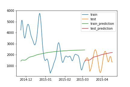
I use auto_arima from python library pmdarima.arima to predict a time series. However, the model seems not work on my data because the prediction results of both training and test data are pretty bad. I would like to know it is because somewhere I did wrong or the data is unpredictable by ARIMA. Here is what I did.

b is my 5-month time series with 700 observations evenly distributed. I first checked if the data is stationary by ADCF.

from statsmodels.tsa.stattools import adfuller

print("Results of Dicky-Fuller Test:")
dftest = adfuller(b, autolag='AIC')

dfoutput = pd.Series(dftest[0:4], index=['ADF Statistic','p-value','#Lags Used','Number of Observations Used'])
for key,value in dftest[4].items():
    dfoutput['Critical Value (%s)'%key] = value

print(dfoutput)

The results are here

-----------------------------------------
Results of Dicky-Fuller Test:
ADF Statistic                   -2.045778
p-value                          0.266868
#Lags Used                       9.000000
Number of Observations Used    690.000000
Critical Value (1%)             -3.439863
Critical Value (5%)             -2.865738
Critical Value (10%)            -2.569005
dtype: float64
-----------------------------------------

It looks a stationary data to me. Then I use auto_arima to find the best parameter combinations and do the fit as well as prediction

from pmdarima.arima import auto_arima

model = auto_arima(b, start_p=1, start_q=1,
                           max_p=6, max_q=6, m=1,
                           seasonal=False,
                           d=0, trace=True,
                           error_action='warn',  
                           suppress_warnings=True, 
                           stepwise=True)
print(model.aic())

model.fit(train)

prediction1 = model.predict(n_periods=len(train))
prediction2 = model.predict(n_periods=len(test))

#plot the predictions for validation set
plt.plot(time_train,train, label='train')
plt.plot(time_test,test, label='test')
plt.plot(time_train, prediction1, label='prediction1')
plt.plot(time_test, prediction2, label='prediction2')
plt.legend()
plt.show()

And the results are

Could anyone please tell me what I did wrong? Thanks! Edit: I understand that the train_prediction curve shown above is actually not the prediction of training data -- it is the predictions of time series len(train) time stamps after the traning data.

Answer 1

You have only 5 months worth of data, I assume observed on daily basis. Your cycle is monthly so m should be 30. Also, your data looks seasonal and therefore should set to true.

Don't try to overfit your data and simply use the default on your first run:

auto_arima(b, error_action='ignore', trace=1,  seasonal=True, m=30)

Answer 2

You did nothing wrong ! ...you probably just didn't read the fine print or understand the assumptions underlying the statistical test you were employing.

See Interrupted Time Series Analysis - ARIMAX for High Frequency Biological Data? for @AdamO's wise reflection that "The correlogram should be calculated from residuals using a model that controls for intervention administration, otherwise the intervention effects are taken to be Gaussian noise, underestimating the actual autoregressive effect."

In other words for auto.arima to be useful you needed to have the following circumstances.

1) a series with no pulses,level shifts,seasonal pulses or deterministic time structure like trends or day-of-the-week effects or day-of-the-month effects or holiday effects et al .

2) a series where the parameters for the underlying arima model are constant over time

3) a series where the error variance of the underlying arima model does not change deterministically at different time points.

Your time series like most have 1 or more of these possible violations, clearly a level/step shift seems to be present BUT only your data knows for sure . If you post your data I will try and help further.

More interesting reading (13) is here https://stats.stackexchange.com/search?q=user%3A3382+AdamO