From a statistical point of view, there are two interesting ideas in this question. The following discussion characterizes them as (1) the behavior of correlations under "tessellation" (which I will define and illustrate) and (2) random-like sampling of circles using a systematic sample. These ideas lead to a proof of a generalized result (stated at the end of this post). It is noteworthy that these ideas are quite different from each other. The first is purely algebraic while the second is an application of the ergodic theory of circular rotations: that's where the randomness lies.
Throughout this post I have made efforts to state and explain only as much as is needed to follow the ideas, with very few discursions--you may wish to fill in some details. I am going to develop the first idea first. Its applicability will only gradually become apparent as we investigate the second idea. Because this idea of tessllating a distribution might be novel, I supply more computational details in the first section.
Correlations and tessellation
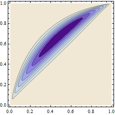
Let $(X,Y)$ be any bivariate random variable, such as the one illustrated here with a contour plot of its density (which is supported in the unit square--but that's not a necessary assumption):

Figure 1. The horizontal axis denotes values of $X,$ the vertical axis denotes values of $Y$, and darker contours represent higher densities.
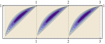
We may translate this random variable any number $i$ to the right by adding $i$ to $X,$ creating the variable $(X+i, Y).$ This shifts the plot of its distribution function (or density, if it has one) $i$ units to the right in the plane. Thus, if we choose a whole number $p$, select $p$ identically distributed and independent versions $(X_i,Y_i),i=0,1,\ldots,p-1,$ and form the mixture of $(X_0,Y_0),$ $(X_1+1,Y_1),\ldots,$ $(X_{p-1}+p-1,Y_{p-1})$ with equal weights, the resulting plot of the distribution looks like $p$ equally spaced copies of that of $(X,Y):$

Figure 2. This illustrates the case $p=3$ applied to the distribution in the first figure. The density contours now, of course, are just $1/3$ as high as before.
Let's call this new variable $(X,Y)_{(p,1)}.$ I call it the "$p$-tessellation of $(X,Y)$ in the $X$ coordinate."
Suppose $(X,Y)$ has finite second moments (which is the mildest condition needed to apply standard correlation formulas) and has correlation $\rho.$
What is the correlation of $(X,Y)_{(p,1)}$?
This has a pretty answer that can be found using basic calculations. For completeness, the details follow, but I invite you to skip directly to the end of this section (to the highlighted lemma) unless you find yourself so sceptical that you need to check the details.
First, represent $(X,Y)_{(p,1)}$ in terms of a variable $U$ that is independent of all the $(X_i,Y_i)$ and has a uniform distribution on the set $\{0,1,\ldots, p-1\}$ as
$$(X,Y)_{(p,1)} = (X_U + U, Y).$$
Writing $E(X,Y)=(\mu,\nu),$ compute
$$\eqalign{
E[(X,Y)_{(p,1)}] &= E[(X_U + U, Y)] = E[E[(X_U + U, Y) \mid U]] \\
&= \sum_{i=0}^{p-1} E[(X_U + U, Y) \mid U=i]\Pr(U=i) \\
&= \frac{1}{p} \sum_{i=0}^{p-1} E[(X_i + i, Y)] \\
&= \frac{1}{p} \sum_{i=0}^{p-1} (\mu + i, \nu) \\
&= \left(\mu + \frac{p-1}{2}, \nu\right).
}$$
To find the second moments, let $\sigma_{xx}=\operatorname{Var}(X),$ $\sigma_{yy} = \operatorname{Var}(Y),$ and $\sigma_{xy} = \operatorname{Cov}(X,Y).$ Using the identity
$$E[((X-\mu) - \alpha)^2] = \sigma_{xx} + \alpha^2$$
for all numbers $\alpha,$ compute
$$\eqalign{
\operatorname{Var}(X_{(p,1)}) &= E[(X_{(p,1)} - (\mu + (p-1)/2))^2) \\
&= \sum_{i=0}^{p-1} E[(X_U + U - (\mu + (p-1)/2))^2 \mid U=i]\Pr(U=i) \\
&= \frac{1}{p}\sum_{i=0}^{p-1} E[(X_i-\mu + i - (p-1)/2)^2 \\
&= \frac{1}{p}\left(\sum_{i=0}^{p-1} \sigma_{xx} + \sum_{i=0}^{p-1} (i - (p-1)/2)^2\right) \\
&= \sigma_{xx} + \frac{p^2-1}{12}.
}$$
In a similar fashion (but more easily),
$$\operatorname{Cov}(X_{(p,1)}, Y_{(p,1)}) = \sigma_{xy}.$$
Finally, it's trivial that
$$\operatorname{Var}(Y_{(p,1)}) = \sigma_{yy}.$$
Applying these results to the formula for correlation, we find
$$\eqalign{
\rho(X_{(p,1)}, Y_{(p,1)}) &= \frac{\operatorname{Cov}(X_{(p,1)}, Y_{(p,1)})}{\sqrt{\operatorname{Var}(X_{(p,1)})\operatorname{Var}(Y_{(p,1)})}} = \frac{\sigma_{xy}}{\sqrt{(\sigma_{xx} + (p^2-1)/12)\ \sigma_{yy}}} \\
&= \rho \sqrt{\frac{\sigma_{xx}}{\sigma_{xx} + (p^2-1)/12}}.
}$$
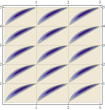
By changing the roles of the $X$ and $Y$ coordinates, for any whole number $q$ we may similarly tessellate $(X, Y)_{(p,1)}$ in the $Y$ direction, creating the $(p,q)$ tessellation of $(X,Y),$ $(X, Y)_{(p,q)}:$

Figure 3. This is a contour plot of the density of the $(3,5)$-tessellation of the density shown in the first figure.
Applying the previous result yields the first result:
Lemma 1. The correlation of the $(p,q)$-tessellation of $(X,Y)$ is $$\rho_{(p,q)}(X,Y) = \rho(X_{(p,q)}, Y_{(p,q)}) = \rho(X,Y) \sqrt{\frac{\sigma_{xx}\sigma_{yy}}{(\sigma_{xx} + (p^2-1)/12)(\sigma_{yy} + (q^2-1)/12)}}.$$
This sometimes simplifies, as it will in the main application later:
Corollary to Lemma 1. When $\sigma_{xx} = \sigma_{yy} = 1/12,$ $$\rho_{(p,q)}(X,Y) = \frac{\rho(X,Y)}{pq}.$$
This corollary is non-vacuous, because you can begin with any random variable $(X,Y)$ with finite moments and rescale its components to make the resulting variances both equal $1/12.$
Sampling circles
The (Euclidean) circle is the topological group $$S^1 = \mathbb{R}/\mathbb{Z},$$ which covers the circle via the map that takes the fractional parts of numbers,
$$\{\ \}:\mathbb{R}\to S^1;\ \{x\} = x - \lfloor x \rfloor.$$
$S^1$ inherits the structure of $\mathbb{R}$ as a measure space and supports Lebesgue integration. As a commutative group it is a $\mathbb Z$-module: whole multiples of elements of $S^1$ are well-defined. Indeed, any point $\{x\}\in S^1$ can be thought of as representing a rotation through an angle of $2\pi \{x\}$ and $n\{x\}$ represents a rotation of $2\pi n \{x\}.$
As in any group, the order of an element $\{x\}$ is the smallest positive integer $n$ for which $n\{x\}=0.$ The order is infinite when no such integer exists. From elementary properties of real numbers it is clear that the rational numbers $\mathbb Q$ are those real numbers $x$ for which $\{x\}$ has finite order in $S^1.$ Letting $q$ be that order, it follows that $x=p/q$ for some integral $p.$
This description affords two conceptual pictures of real numbers $x$ when interpreted as elements of $S^1:$ $x$ can be viewed as a point on the circle or as an action on the circle via rotation, whereby $T_x:S^1\to S^1$ maps $\{y\}$ to $\{x+y\}.$ This action forms a dynamical system of the iterates of $T_x$ and its inverse $$(\ldots, T_x^{-1}, T_x^0, T_x^1,T_x^2, \ldots) = (\ldots, T_{-x}, T_0, T_{x}, T_{2x}, \ldots)$$ on the circle.
A fundamental result of ergodic theory asserts that when $x$ is irrational--that is, when all the transformations in this system are distinct--the images of any point eventually fill out the circle uniformly. That is, let $0\le a\le b \le 1$ designate any interval $(\{a\}, \{b\}]$ on $S^1$ of length $b-a.$ Beginning with any point $p\in S^1,$ form the systematic sample $$\mathcal{S}(p,n) = p=T_x^0(p), \{x\}+p = T_x(p), 2\{x\}+p = T_x^2(p), \ldots, (n-1)\{x\}+p = T_x^{n-1}(p)$$ of length $n.$ The empirical distribution of these points assigns the probability $k/n$ to the interval where $k$ is the number of the sample points that lie within it:
$$\eqalign{\mu_{p,n}(a,b) &= \frac{1}{n} \#\{i\mid 0\le i \lt n\text{ and }T_{ix}(p) \in (\{a\}, \{b\}]\} \\&= \frac{1}{n} \# \{i \mid 0 \le i \lt n\text{ and } \{a\} \lt \{ix\} \le\{b\}\}.}$$
The ergodic theorem implies that for any given $a$ and $b$ this fraction has a limit as $n$ grows large and that limit is the length of the interval,
$$\lim_{n\to\infty} \mu_{p,n}(a,b) = b-a.$$
In more statistical language,
When we systematically sample the circle by starting at any fixed point $p$ and step off in equal steps of size $dt$, then either (a) the sample starts repeating itself endlessly when $dt$ has finite order or otherwise (b) when it is sufficiently large, it provides an excellent approximation to the uniform probability distribution on the circle.
A torus is the product of two circles, $T^2 = S^1 \times S^1 = \mathbb{R}^2 / \mathbb{Z}^2.$ Its points are ordered pairs $(\{x\}, \{y\})$ of points on the circle. As a geometrical object it is flat and its geodesics through a point $(x_0, y_0)$ are all images of lines in $\mathbb{R}^2,$ which can therefore be parameterized in the form
$$\gamma_{(\xi,\eta);(x_0,y_0)}:\mathbb{R}\to T^2,\ \gamma_{(\xi,\eta);(x_0,y_0)}(t) = (\{x_0 + t\xi\}, \{y_0 + t\eta\}).$$
Such lines originate at the base point $(x_0,y_0)$ and move at a speed of $\sqrt{\xi^2 + \eta^2}$ in the direction given by the vector $(\xi, \eta).$ When $\xi$ and $\eta$ are rationally related and not both zero--that is, when there are integers $p$ and $q$ with $q\xi = p\eta,$ the image of this geodesic is a circle because
$$\gamma_{(\xi,\eta);(x_0,y_0)}\left(\frac{q}{\xi}\right) = (\{x_0 + q\}, \{y_0 + p\}) = (\{x_0\}, \{y_0\})$$
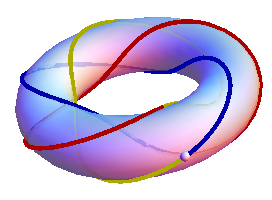
returns to the starting point, heading in the initial direction. (If $\xi=0,$ set $t=q/\eta$ in the preceding calculation). When $p$ and $q$ have no common divisors, $t=q/\xi$ is the first time the geodesic returns to its origin. The image is a $(p,q)$ Torus knot, which can be illustrated with this distorted (non-flat) torus:

Figure 4. The base point $(x_0,y_0)$ is shown as a white ball. The image of the geodesic first traces the blue curve, where it travels once around the torus while twisting $5/3$ of the away around; then it traces the red curve while twisting another $5/3$ of the way; and finally it traces the gold curve with a twist of $5/3$ to return to the start, about to head off in the original direction. The entire trip goes around the torus $p=3$ times while twisting $q=5/3+5/3+5/3=5$ times.
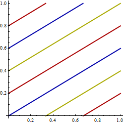
The same path can be more clearly shown--albeit with visual breaks--in the coordinate system of $T^2,$ which is the square $[0,1)\times [0,1)$ designating all ordered pairs of fractional parts of real numbers:

Figure 5. The base point is at the origin, $(0,0).$ Coloring is the same as previously. The knot proceeds along the blue line to the point $(1,3/5)$ which is equivalent to $(0,3/5)$, where it reappears and travels to the point $(5/3,1)$, equivalent to $(5/3,0),$ where it reappears. At this point it has traversed the vertical direction once and the horizontal direction $5/3$ times. The geodesic continues in like manner through the red and gold curves, returning to the origin at the upper right corner, where $(1,1)$ is equivalent to $(0,0).$
When the image of a geodesic is a circle, the ergodic theorem applies: we may systematically sample it by starting at its origin and stepping out equal distances $dt$, provided $dt$ is not a rational fraction of the length of the circle.

Figure 6. The gray lines in all four panels depict the same geodesic as before. Starting at the origin, points in the panel at left have been spaced equally along the geodesic--coloring them as before to help the eyes keep track--until the origin has first been crossed (where the color turns to green). The even spacing is a crude but decent approximation to the uniform distribution along the geodesic. The next panels repeat this process, showing how the points fill the geodesic more and more densely as the sample size grows. As is evident in the second panel from the left, the points might not be very uniform over small distances, but the progression from left to right shows how those local non-uniformities eventually get smoothed out.
Statement and proof of the results
The dashed lines in Figure 6 are drawn to remind you of figures 2 and 3, showing tessellated distributions. Indeed, it should be clear that such a diagram of any $(p,q)$ torus knot originating at $(x_0,y_0)=(0,0)$ can be subdivided into $pq$ similar rectangles along the vertical lines at $0, 1/p, 2/p, \ldots, 1$ and the horizontal lines at $0, 1/q, 2/q, \ldots, 1.$ This exhibits the uniform distribution along the knot as a tessellation of the uniform distribution along the diagonal of the bottom left rectangle.
We have the desired result, once we make a few more mopping-up observations, all of which are obvious (I hope) and easily proven:
The uniform distribution along the diagonal of a rectangle has uniform marginals and correlation coefficient $1.$
The correlation coefficient $\rho(X,Y)$ is unchanged when $X$ and $Y$ are separately rescaled. Thus, for the purpose of computing correlations in Figure 6 we may assume the scales are such that all the rectangles are actually unit squares.
The variance of the uniform marginal on a unit square is $1/12.$
Consequently, the corollary to Lemma 1 implies the correlation coefficient of the uniform distribution on a geodesic that forms this $(p,q)$ knot is $1/(pq).$
The ergodic theorem implies the correlation coefficient of a systematic sample of a geodesic approaches the correlation of the uniform distribution along that geodesic as the sample size grows.
The correlation of the systematic sample is precisely the correlation as defined in the question.
The geodesics that are not circles are one-to-one images of lines: the ergodic theorem implies they fill the torus uniformly. Thus, the limiting distribution of a systematic sample of such a geodesic (no matter what its spacing may be) is the uniform distribution on the torus. Its bilateral symmetry implies its correlation coefficient is zero.
Just one more calculation is needed: the length of $\gamma_{(\xi,\eta);(x_0,y_0)}$ when $q\xi = p\eta.$ But this is the locally isometric image of a line in $\mathbb{R}^2.$ It first returns to its origin when $\gamma_{(\xi,\eta);(x_0,y_0)}(t) = (x_0, y_0),$ which is the smallest positive $t$ for which both $t\xi$ and $t\eta$ are integers. Assuming $p$ and $q$ are relatively prime and $\xi\ne 0,$ that is $t = q/\xi.$ Since the geodesic is traversed at a constant speed of $\sqrt{\xi^2+\eta^2},$ its length is $q\sqrt{\xi^2+\eta^2}/\xi.$ (When $\xi=0,$ its length is $1.$)
Putting these results together and specializing to an origin of $(0,0)$ (simply to avoid complicating the statements), we conclude the following:
Let $\xi$ and $\eta$ be real numbers, not both zero. Let $dt$ be a positive number and form the ratio $$\lambda(dt;\xi,\eta)=\frac{dt}{\sqrt{1+(\eta/\xi)^2}}$$ (set to $1$ when $\xi=0$).
For each $n\gt 1,$ construct the sequence $\rho_n$ of empirical correlation coefficients of the systematic sample data $(\{i\, dt\, \xi\}, \{i\, dt\,\eta\,\}),$ $i=0, 1, \ldots, n-1.$
- When there are no rational numbers $p$ and $q$ for which $q\xi=p\eta,$ $$\lim_{n\to\infty}\rho_n = 0.$$
- Otherwise, when $\lambda(t;\xi,\eta)$ is irrational, let $p$ and $q$ be relatively prime integers for which $q\xi=p\eta.$ Then $$\lim_{n\to\infty}\rho_n = \frac{1}{pq}.$$
Applying this result to $\xi=1,\eta = b^k$ produces the speculated conclusions of the question. Except as explicitly described in (1), there are no special exceptions. In particular, when $b$ is irrational conclusion $(1)$ applies and otherwise the only numbers $dt$ ("$x$" in the question) that do not yield result $(2)$ are the rational multiples of $\sqrt{1+b^{2k}}.$
(This result omits the case of systematically sampling a $(p,q)$ knot by a rational fraction of its length. Such samples repeat their elements over and over and so clearly attain limits. It's a simple, although potentially fussy, question of arithmetic to work out what the limiting correlations are. They can differ greatly from $1/(pq);$ they needn't even have the same sign.)
Finally, it's a simple exercise to work out the answer for geodesics at arbitrary origins: the uniform geodesic distribution within the bottom left rectangle no longer has $\rho=1,$ but it is readily computed and will multiply $1/(pq)$ according to Lemma 1.

