How do I define an "interaction" contrast with single explantory variable?

Question

Suppose I have an experiment with four groups defined by two binary variables.

|       | Control | Treatment |
|-------|---------|-----------|
| Men   | M.C     | M.T       |
| Women | W.C     | W.T       |

I want to model the interaction between treatment effect and sex. In particular, I want to know what the treatment effect is for women and for men, and my question to you regards the difference between treatment effect in men vs. in women.

I can write the model in these two ways (among others):

1. Y ~ 1 + Sex + Drug + Sex:Drug
2. Y ~ 0 + Sex.Drug, where I define Sex.Drug as a categorical variable taking the values indicated in the table above.

In the first case, testing the Sex:Drug term is the answer I'm looking for. In the second case, I'm not certain, and I haven't found a simple explanation anywhere on the internet. (There are statistical tools that make the single-categorical-variable parameterization much more convenient for me.)

I believe the answer is relatively straightforward: the contrast M.T - M.C tests treatment effect in men, and W.T - W.C tests in women, so (M.T - M.C) - (W.T - W.C) == M.T + W.C - M.C - W.T seems like it should work. Is that correct?

I have two further questions for extra credit:

1. How can I prove mathematically that the different model parameterizations and associated contrasts are equivalent?
2. What is a reference that teaches this stuff? (Preferably on the internet, but I'll take what I can get.)

Thanks!

Answer 1

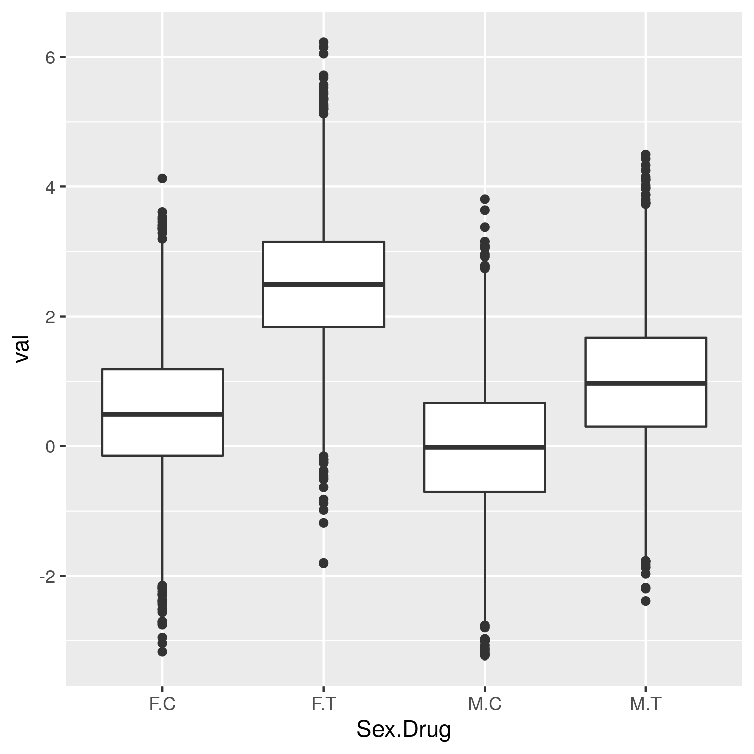
Yes, they are equivalent, at least if the following numerical test is generally representative.

library(lsmeans)
library(dplyr)
library(ggplot2)

set.seed(1)
n <- 5000 ## per condition
dat <- data.frame(Sex=rep(c("M", "F"), 2*n), Drug=rep(c("C", "T"), each=2*n))
dat$Sex.Drug <- paste(dat$Sex, dat$Drug, sep=".")

meanz <- c("M.C"=0, "M.T"=1, "F.C"=0.5, "F.T"=2.5)
dat$val <- rnorm(nrow(dat), mean=meanz[dat$Sex.Drug])

ggplot(dat, aes(x=Sex.Drug, y=val)) + geom_boxplot()

dat %>% group_by(Sex, Drug) %>% summarize(mean(val))

# A tibble: 4 x 3
# Groups:   Sex [2]
  Sex   Drug  `mean(val)`
  <fct> <fct>       <dbl>
1 F     C          0.513 
2 F     T          2.50  
3 M     C         -0.0261
4 M     T          0.992 

Let's first identify what the true answer we're expecting is. The question is, what's the difference in drug effect in men vs. women. In men, the drug effect is, 1 - 0 = 1, while for women, the drug effect is 2.5 - 0.5 = 2. So the true answer is 1 - 2 = -1.

Now here's the first model:

lm1 <- lm(val ~ 1 + Sex + Drug + Sex:Drug, data=dat)
print(summary(lm1))

Call:
lm(formula = val ~ 1 + Sex + Drug + Sex:Drug, data = dat)

Residuals:
    Min      1Q  Median      3Q     Max 
-4.3026 -0.6732 -0.0111  0.6742  3.8364 

Coefficients:
            Estimate Std. Error t value Pr(>|t|)    
(Intercept)  0.51303    0.01416   36.22   <2e-16 ***
SexM        -0.53914    0.02003  -26.91   <2e-16 ***
DrugT        1.98674    0.02003   99.18   <2e-16 ***
SexM:DrugT  -0.96879    0.02833  -34.20   <2e-16 ***
---
Signif. codes:  0 ‘***’ 0.001 ‘**’ 0.01 ‘*’ 0.05 ‘.’ 0.1 ‘ ’ 1

Residual standard error: 1.002 on 19996 degrees of freedom
Multiple R-squared:  0.4687,    Adjusted R-squared:  0.4686 
F-statistic:  5880 on 3 and 19996 DF,  p-value: < 2.2e-16

And here's the second:

lm2 <- lm(val ~ 0 + Sex.Drug, data=dat)
lsm2 <- lsmeans(lm2, "Sex.Drug")
print(names(lm2$coefficients))

contr <- list(SexM=c(-0.5, -0.5, 0.5, 0.5),
              DrugT=c(-0.5, 0.5, -0.5, 0.5),
              SexM.DrugT=c(1, -1, -1, 1))
print(contrast(lsm2, contr))

 contrast   estimate     SE    df t.ratio p.value
 SexM         -1.024 0.0142 19996 -72.261 <.0001 
 DrugT         1.502 0.0142 19996 106.065 <.0001 
 SexM.DrugT   -0.969 0.0283 19996 -34.198 <.0001 

You'll see that the estimate for SexM.DrugT under model 2 is identical to the estimate for the estimate for SexM:DrugT under model 1, with identical t statistics. So, the answer to my main question is, yes, the two parameterizations produce equivalent regressions.

One thing that wasn't obvious to me was why the SexM and DrugT contrasts from model 2 weren't identical to the coefficients sharing those names in model 1. The answer is that in the first model, the SexM explanatory variable does not quantify the mean difference between val across sexes. It quantifies the difference between sexes in the absence of treatment effects. Perhaps this is obvious to many of you, I feel like it should've been obvious to me, but it wasn't. (Indeed, this a very good thing because it means we can "regress out" confounding factors.)

print(contrast(lsm2, list("SexM_only"=c(-1, 0, 1, 0))))

 contrast  estimate   SE    df t.ratio p.value
 SexM_only   -0.539 0.02 19996 -26.915 <.0001 

I'm still interested in the extra credit! And, in fact, this answer provokes the additional question of how to write the contrast for the second model that answers the question answered by the first o