Detrending inputs still produces uncorrelated residuals but Durbin Watson is still low

Question

I have two time series, and I am using one to forecast the other. Both are trend-nonstationary, so I de-trended them. The resulting model produces non-autocorrelatated residuals, but the Durbin-Watson is still low.

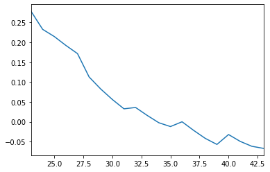
First, my independent variable is plotted, and I see that it is trend-nonstationary.

I can test and see that it is indeed trend-nonstationary, and that a removal of a trend would yield a stationary series.

from statsmodels.tsa.statstools import adfuller

df_temp['past_flow'].plot()
plt.show()
plt.hist(df_temp['past_flow'])
plt.show()
result = adfuller(df_temp['past_flow'])
print('ADF Statistic: %f' % result[0])
print('p-value: %f' % result[1])

ADF Statistic: -3.711959

p-value: 0.003948

So I detrend the series

df_temp['past_flow'] = signal.detrend(df_temp['past_flow'] )

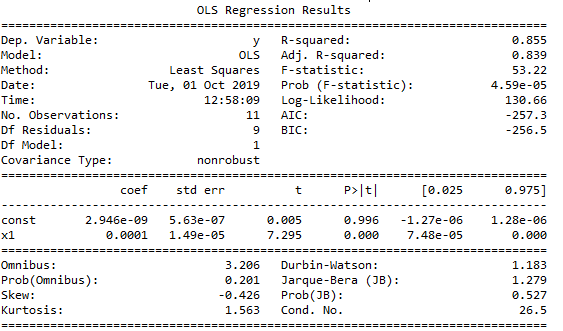
I do the same with my dependent series, and I yield the following model:

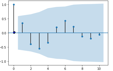
This model has a rather low Durbin-Watson, but plotting the residuals, I see no autocorrelation:

Answer 1

Just because Y and X are non-stationary (themselves) , this doesn't necessarily imply that a useful causative model couldn't simply be Y(t)=b0 + b1*X(t) or something more complex incorporating lags of X or arima structure or latent deterministic effects like pulses,level shifts,seasonal pulses or local time trends.

With 11 observations one has to tread very very very gently.

SOME COMMENTS ABOUT THE GENERAL APPROACH OF CAUSAL MODEL IDENTIFICATION

Detrending or differencing one or more series can be useful to IDENTIFY a possible useful model see http://www.autobox.com/pdfs/WHY-WE-FILTER.ppt . This is generally referred to as the pre-whitening step to tentatively transform data that has an auto-correlated predictor to one that does not , in order to use subsequent cross-correlations (impulse-response weights) to IDENTIFY the relationship between the original series https://autobox.com/pdfs/PREFERRED.pdf and here http://viewer.zmags.com/publication/9d4dc62a#/9d4dc62a/66 for some rigorous critique and bullet-proof testing of the approach.