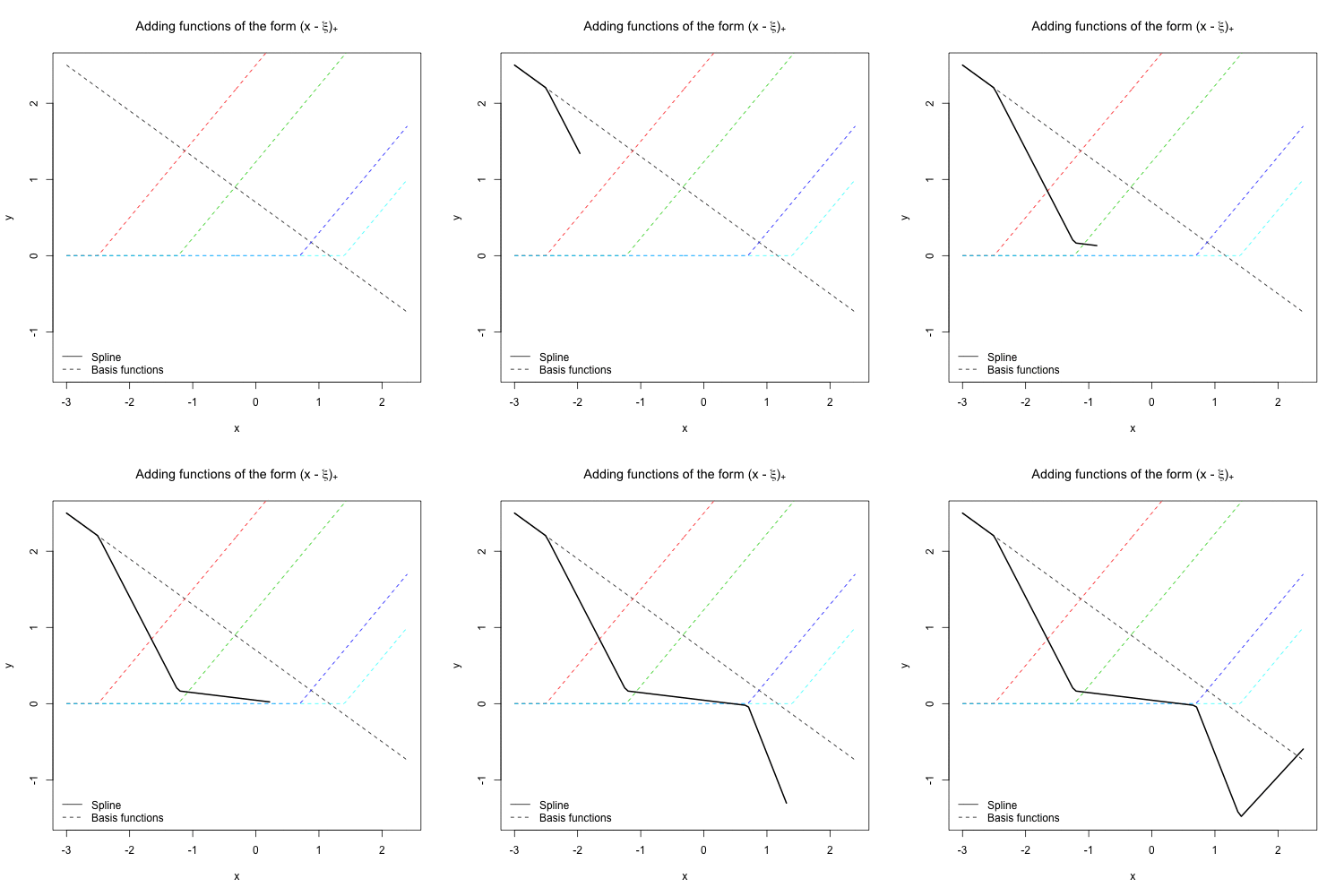
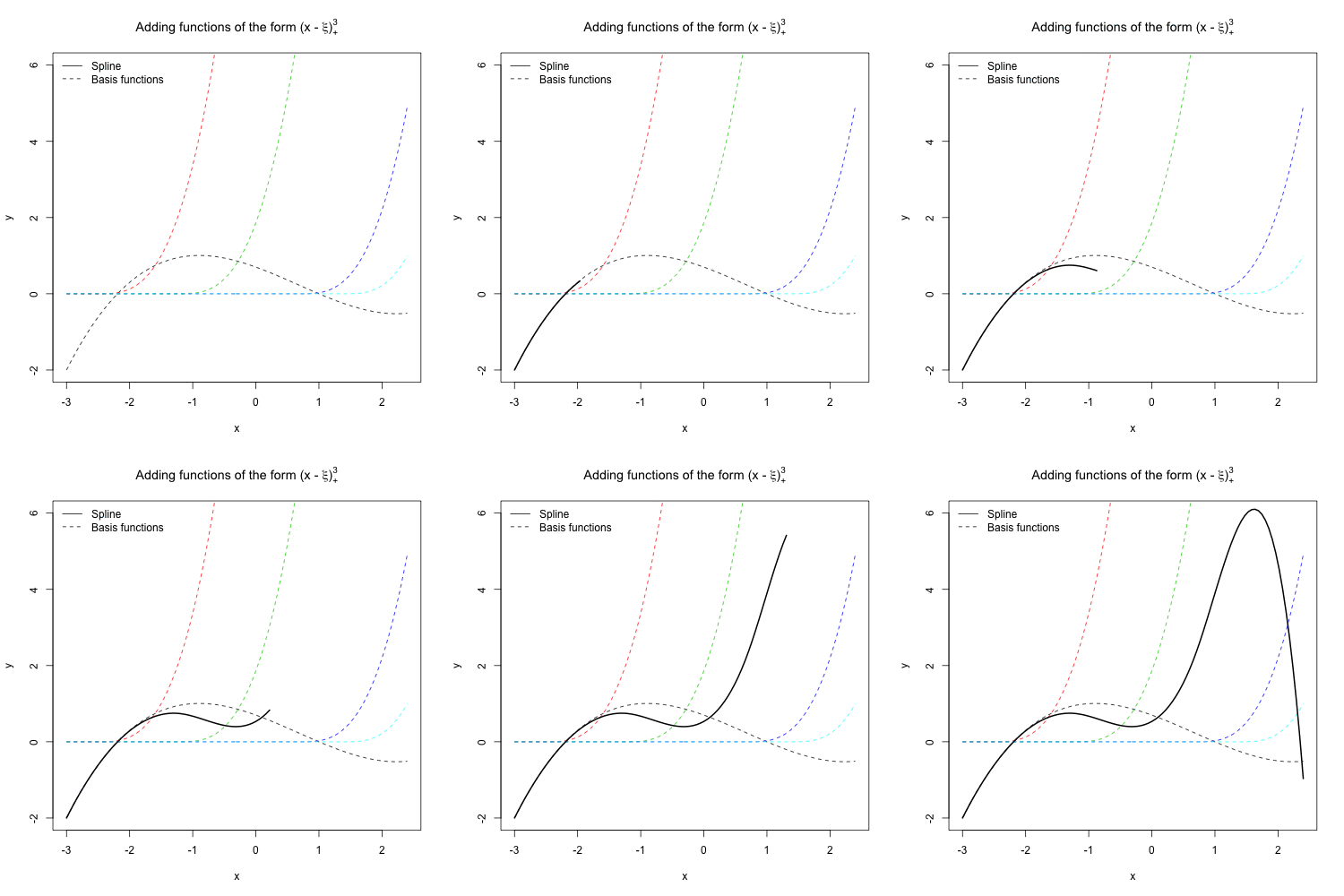
I know splines use basis functions to approximate a function locally, so that the function in one region is approximated with a weighted sum of these basis functions. Suppose the input is one-dimensional and suppose we use $h$ to indicate the basis functions and $\beta$ for the coefficients in one region we have:
$$y(x) = \sum_{i=0}^N h_i(X) \beta_i$$
For example, assuming a first order polynomial we can use a constant basis function $h_0(X) = 1$ and a first order function $h_1(X) = X$. The sum becomes:
$$y(x) = \sum_{i=0}^1 h_i(X) \beta_i =\beta_0 h_0(X)+\beta_1 h_1(X) = \beta_0+\beta_1 X $$
In the region $j$ we can approximate the function as:
$$f_j(x) = \beta_{j,0} + \beta_{j,1} X$$
and in the region $j+1$:
$$f_{j+1}(x) = \beta_{j+1,0} + \beta_{j+1,1} X$$
To force continuity at the knot (or boundary) point $\xi$:
$$\beta_{j,0} + \beta_{j,1} \xi = \beta_{j+1,0} + \beta_{j+1,1} \xi$$
In the Elements of Statistical Learning book it is said:
A more direct way to proceed in this case is to use a base that incorporates the constraints $h_2(X)=(X-\xi)_+$ where $t_+$ denotes the positive part.
I don't understand this notation and how it fits into the previous one with the sum: what does the sum becomes? Is it something like that?
$$f_j(x) = \beta_{j,0} h_0(X)+ \beta_{j,1} h_1(X)+ \beta_{j,2} h_2(X)=\\ =\beta_{j,0} + \beta_{j,1} X+ \beta_{j,2} (X-\xi)^+ = \\= \beta_{j,0} + \beta_{j,1} X+ \beta_{j,2} X -\beta_{j,2} \xi^+ $$
and in the region $j+1$:
$$f_{j+1}(x) = \beta_{j+1,0} h_0(X)+ \beta_{j+1,1} h_1(X)+ \beta_{j+1,2} h_2(X)=\\ =\beta_{j+1,0} + \beta_{j+1,1} X+ \beta_{j+1,2} (X-\xi)^+ = \\= \beta_{j+1,0} + \beta_{j+1,1} X+ \beta_{j+1,2} X -\beta_{j+1,2} \xi^+ $$
How does this expression embed the constraint?


