5
$\begingroup$

Let $F_i:\mathbb R\to[0,1]$ be a distribution function$^1$ and $$F_i^{-1}(t):=\inf\left\{x\in\mathbb R:F_i(x)\ge t\right\}\;\;\;\text{for }t\in[0,1].$$

I've got a computer program where only $F_i^{-1}$ (not $F_i$) is directly available. Assume $t_1\in[0,1]$ and $x:=F_1^{-1}(t_1)\in F_2^{-1}([0,1])$. I need to compute a $t_2\in[0,1]$ such that $x=F_2^{-1}(t_2)$. How can I do this?

First of all, we know that $$\left\{t_2\in[0,1]:F_2^{-1}(t_2)=x\right\}=\begin{cases}[F_2(x-),F_2(x)]&\text{, if }F_2\text{ is continuous at }x\text{ or }\forall y<x:F_2(y)<F_2(x-)\\(F_2(x-),F_2(x)]&\text{, otherwise}.\end{cases}$$

Now, I've read (here in section 6.1) the following, but can't really make sense of it: Assuming that $F_2^{-1}([a,b])=\{x\}$ for some $0\le a\le b\le 1$ we can find $t_2$ by sampling $u$ with uniform distribution on $[0,1]$ and set $t_2:=a+(b-a)u$. Why does this work? And if it works, how can we apply it in practice (i.e. how do we find $a,b$)?

Remark: I think this book page (above Example 3.31) is related.


$^1$ i.e. $F_i$ is right-continuous and nondecreasing with $F(-\infty):=\lim_{x\to-\infty}F(x)=0$ and $F(\infty):=\lim_{x\to\infty}F(x)=1$.

$\endgroup$
5
  • 1
    $\begingroup$ Don't reinvent the wheel (unless you are expert on numerical analysis): just apply a root finder to the function $t \to F_2^{-1}(t) - x.$ Would "ambigious" in the title mean "ambiguous"? What would an "ambiguous interval" mean? $\endgroup$
    – whuber
    Commented Jan 6, 2020 at 19:58
  • $\begingroup$ @whuber (a) Actually, I don't know what you mean by a "root finder", but please assume that just a single evaluation of $F_2^{-1}$ is computationally expensive. (b) It should be "ambiguous". And I have no idea what "ambiguous Intervals" are. I've just copied the section 6.1 in the reference. I guess they simply mean that there is not a unique number $t$ in the interval $[a,b]$ such that $F_2^{-1}(t)=c$. $\endgroup$
    – 0xbadf00d
    Commented Jan 6, 2020 at 20:24
  • $\begingroup$ Root finders are subroutines to find roots of equations. Your choice of method ought to depend on properties of the function. In your case, a simple bisection method will work well and requires very few evaluations of the function. The more you know about the function, the more efficient you can be. Please refer to any numerical analysis text for details (Numerical Recipes is very good for this). $\endgroup$
    – whuber
    Commented Jan 6, 2020 at 21:14
  • $\begingroup$ @whuber I think the issue is more with the case of an atom at $x$, in which case numerical root finders are not helpful. $\endgroup$
    – Xi'an
    Commented Jan 6, 2020 at 21:22
  • $\begingroup$ @X`ian The bisection method, properly implemented, will work fine: that's why I recommended it. $\endgroup$
    – whuber
    Commented Jan 6, 2020 at 21:49

1 Answer 1

3
$\begingroup$

The bisection method is guaranteed to work even for such discontinuous $F^{-1},$ provided it is suitably implemented.

Here is pseudocode (that actually works in R):

function(f, x, tol=1e-8, ...) {
  u <- 1
  l <- 0
  repeat {
    m <- (u + l) / 2
    if (f(m, ...) - x <= 0) l <- m else u <- m
    if (u - l <= tol) break # (See the end of this post for a better test)
  }
  return(u)
}

The arguments are (1) the name of $F^{-1},$ (2) the value of $x,$ (3) a positive error tolerance (the result will be accurate to this amount), and (4) any other arguments that need to be passed to $F^{-1}.$ I will refer to this function as findroot.

Before proving this works, let's look at how it might be used, again using R.

> findroot(qpois, 2, tol=0, lambda=2)
[1] 0.6766764

qpois is the Poisson percentile function. Thus, with $\lambda=2$ we hope that

$$0.6766764 = e^{-\lambda}(1 + \lambda + \lambda^2/2!)$$

and indeed that's the case. This figure plots part of $F^{-1},$ showing $x$ as a horizontal dashed line and the solution as a vertical red line:
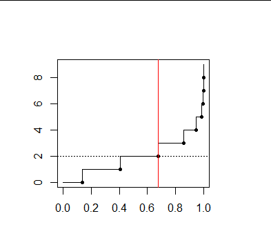
Figure

Let's turn to proving this works. Let $\epsilon \ge 0$ be the tolerance. Consider the proposition

$$\mathcal{P}_{x}(l,u):\ F^{-1}(l) - x \le 0 \le F^{-1}(u) - x\quad \text{ and }\quad u^\prime > u \implies F^{-1}(u^\prime) - x \gt 0. $$

If we take the values of $F^{-1}$ at any number greater than $1$ to be $\infty,$ then $\mathcal{P}_{x}(0,1)$ is true. Assuming hypothetically $\mathcal{P}_{x}(l,u)$ at the beginning of the loop, note that $u$ will be decreased to $u^\prime$ only when $F^{-1}(u^\prime) - x \gt 0$ and in any event $F^{-1}$ changes sign between the new $l$ and new $u.$ Thus, $\mathcal{P}_{x}(l,u)$ remains true at the end of the loop. After exiting, $u$ and $l$ are within $\epsilon$ of each other and $\mathcal{P}_{x}(l,u)$ remains true (by induction). Thus, the value $t = u$ returned by findroot enjoys two properties:

$$F^{-1}(t-\epsilon)-x \le 0 \lt F^{-1}(t) - x.$$

That's what it means for $t$ to be within $\epsilon$ of a solution to $x = F^{-1}(t),$ QED.

Notice that after $n$ iterations of the loop, the difference $u-l = 2^{-n}.$ Therefore this procedure terminates after $\lceil -\log_2 \epsilon \rceil$ iterations. That's a reasonably sparing use of calls to $F^{-1}.$


In a practical application, the test u - l <= tol is too naive about floating-point roundoff error: if tol is very small (but still positive), this condition might never hold. One way to guarantee termination is to set an upper limit on the number of iterations; $52$ will be fine for double-precision arithmetic. A slightly more flexible solution in R uses zapsmall, as in

    if (zapsmall(c(u - l, 1))[1] <= tol) break

When $u-l$ is indistinguishable from $0$ compared to $1,$ it is set to $0,$ guaranteeing termination of the loop.

$\endgroup$
11
  • $\begingroup$ Thank you for your answer, I guess it fits the problem well. However, in my actual application $F_i$ is actually a mapping from $\mathbb R^k\to[0,1)^d$, where $k$ something between $6$ and $100$. Can we generalize your solution or come up with a more sophisticated approach? $\endgroup$
    – 0xbadf00d
    Commented Jan 10, 2020 at 16:34
  • $\begingroup$ Could you explain in what sense this could be construed as a "distribution function" when $d \gt 1$? $\endgroup$
    – whuber
    Commented Jan 10, 2020 at 16:37
  • $\begingroup$ Yes: What I mean is that I've got a Borel measurable transformation $\varphi$ between $[0,1)^d$ and $M^k$ such that $\left.\lambda\right|_{[0,\:1)}^{\otimes d}\circ\varphi^{-1}=q\mu$, where $\lambda$ is the Lebesgue measure on $\mathcal B(\mathbb R)$, $M\subseteq\mathbb R^3$ is a 2-dimensional manifold and $\mu$ is a measure on $\mathcal B(M)$. In some sense, $\varphi$ is the inverse cdf. $\endgroup$
    – 0xbadf00d
    Commented Jan 10, 2020 at 16:51
  • $\begingroup$ Because by definition the values of a CDF (even defined on a manifold) are in the interval $[0,1],$ I cannot make any sense of this when $d\ne 1.$ $\endgroup$
    – whuber
    Commented Jan 10, 2020 at 16:53
  • $\begingroup$ Please take a look at the reference in the question: cs.dartmouth.edu/~wjarosz/publications/bitterli18reversible.pdf. It is described on the bottom of the left side (Primary Sample Space MLT). What I called $\varphi$, they call $S$. $\endgroup$
    – 0xbadf00d
    Commented Jan 10, 2020 at 16:55

Your Answer

By clicking “Post Your Answer”, you agree to our terms of service and acknowledge you have read our privacy policy.

Not the answer you're looking for? Browse other questions tagged or ask your own question.