Interval Estimation for a Binomial Proportion Given a Specific Test Outcome

Question

Imagine that I had a coin, I tossed it 10 times (n) and it came up heads each time (x). What proportion heads I would get if I tossed it infinity times? A point estimate is 100%.

I can get the confidence intervals (CI) from:

low, high = statsmodels.stats.proportion.proportion_confint(10, 10, alpha=A, method='jeffreys')

& I can get the coverage probability of the 95% CI (CP) from:

coverage = binom.coverage(p, 10, method="bayes", type = "central")$coverage

&:

coverage = binom.coverage(p=0.5, n=10, conf.level=C_L, method="bayes", type="central")$coverage

gives:

The CP calculation uses n but doesn't consider x. Can I combine the CI and CP results to get a distribution of the CP for this case please, where x is known? And would this be an appropriate method to use for the comparison of techniques for constructing CIs?

Answer 1

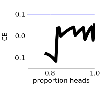
x=10 n=10

Use the 95% CI of the proportion heads, [0.783, 1], according to the Jeffreys equal tailed interval. For the given value of n, calculate CP for an equally spaced range of 30 values of the proportion heads that lie within this CI:

If we define:

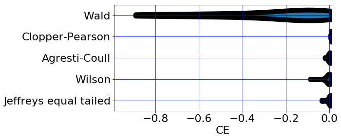
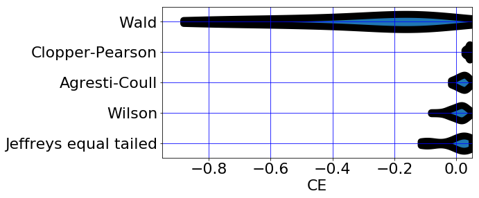
Coverage Error (CE) = CP - CL

Then the method with the CE distributed the most tightly about zero is the best. For this case the best method compared is Agresti-Coull:

This method of comparison makes the simplifying assumption that the proportion heads is equally likely to lie anywhere within the 95% CI and that it does not lie outside of it.

Here is a Python script that works for any n, x and CI:

import statsmodels.api
from rpy2.robjects.packages import importr
binom = importr('binom')
from rpy2 import robjects
import matplotlib.pyplot as plt

n = 10 # samples
x = 10 # positive results
CI = 0.95 # confidence level
methods = ["'bayes', type='central'",
           "'wilson'",
           "'agresti-coull'",
           "'exact'",
           "'asymptotic'"]
LW = 10 # line width

# CI
low, high = statsmodels.stats.proportion.proportion_confint(x, n, alpha=1-CI, method='jeffreys')
if x == 0: low  = 0
if x == n: high = 1

# CP
step = (high - low) / 31

robjects.globalenv["LV"] = robjects.r(low)
robjects.globalenv["HV"] = robjects.r(high)
robjects.globalenv["SV"] = robjects.r(step)
robjects.globalenv["CV"] = robjects.r(CI)

CP = {}

for method in methods:
    r_string = """library(binom)
    p = seq(LV,HV,SV)
    coverage = binom.coverage(p, 10, conf.level = CV, method=TECHNIQUE)$coverage
    """.replace('TECHNIQUE',method)
    robjects.r(r_string)
    R_C = list(robjects.r['coverage'])
    CP[str(method)] = R_C

R_P = list(robjects.r['p'])

# Coverage Error (CE) = CP - CI
CE = {}
for method in methods:
    CE[str(method)] = [x - CI for x in CP[str(method)]]

# Dict to Lists
labels, data = [*zip(*CE.items())]

# Plots    
font = {'weight' : 'normal',
        'size'   : 22}
plt.rc('font', **font)

# Violin
fig, ax = plt.subplots()
parts = plt.violinplot(data, showextrema=False, vert=False)

for pc in parts['bodies']:
    pc.set_edgecolor('black')
    pc.set_alpha(1)
    pc.set_linewidth(LW)

plt.xlabel('CE')
fig.set_size_inches(8,4)
#plt.xlim([-.05,.05])
plt.xlim([-CI,1-CI])

# Override the method names
labels=(['Jeffreys equal tailed','Wilson','Agresti-Coull','Clopper-Pearson','Wald'])

plt.yticks(range(1, len(labels) + 1), labels)

plt.grid(b=True, which='major', color='b')
plt.show()

After checking it for the 95% CI, check it for the 99% CI as well to see whether the tails are equal: