Which statistical analysis should I perform if the data sets are not normally distributed?

Question

I am doing an experiment where there are two independent groups; one is the group of "infected" patients another is the group of "sepsis" patients. I am comparing "platelet monocyte aggregates(PMA)" data in between the two groups. As PMA is a scale data I thought of doing an independent sample T test. But when I tested for normality and equality of variance I found that my data were not normally distributed but they have equal variance. The sample size of both the group are also not equal; one group has 71 samples and the other group has 26 samples. So I did both independent T test with bootstrapping and Mann Whitney U test to compare the mean in between the two groups. But I got p value which is not significant by Independent T test and a p value which is significant by Mann Whitney U test. I read somewhere that as Mann Whitney U test is a non parametric test it has less power. So should I prefer Independent T test with bootstrapping? Or may be I am wrong somewhere. I am not a statistics student, I am a Medical student. So statistics knowledge is very limited. So kindly excuse me if I am wrong and suggest me a solution. Thank you.

Answer 1

About the t-test

With a t-test you are considering whether the means of two distributions are significantly different or not, by comparing the means of samples from those two distributions.

For sufficiently large samples the value $d = \bar{x_1} - \bar{x_2}$ is approximately Gaussian distributed with some mean $\mu_d$ and $\sigma_d$ and the normalized/standardized value $z= (\bar{x_1} - \bar{x_2})/\sigma$ can be used to test the hypothesis that $\mu_d=0$. (and if the samples are drawn from a normal distribution, then $d$ will be exactly normal distributed)

The value $\sigma_d$ is often unknown and estimated based on the data giving an estimate $\hat\sigma_d$ of the standard deviation of the difference in sample means . So we do not really compute $z=(\bar{x_1} - \bar{x_2})/\sigma$ but instead $t=(\bar{x_1} - \bar{x_2})/\hat\sigma$. The distribution of $t$ does not follow a normal distribution like $z$. If the samples are normally distributed with equal standard deviation then $t$ will be following a t-distribution.

But if the samples are not normally distributed then this will not be the case.

However, if the sample size is large then the distribution will approximate a normal distribution a lot (because the distribution in $\hat\sigma$ is getting more narrow and the distribution in $d$ is getting more like a normal distributed variable). How large the sample needs to be depends on the way how the population distribution deviates from the normal distribution. If the population has large outliers then $d$ will not approach a normal distribution quickly. But if the population is more like a truncated distribution, then the sample will approach a normal distribution quickly.

Example/demonstration

See the below demonstration for the difference in three different population distributions: the normal distribution, a uniform distribution (representing low kurtosis), and a t-distribution (representing high kurtosis). When you have samples of size 50 then there is hardly and difference.

In the image below you see the joint distribution of 1: the estimate of the pooled standard deviation 2: the difference in the means. The t-test draws two boundaries, in this case excluding 5% of the points on the left and right. These boundaries are diagonal. The values $-1.984 \hat\sigma < \bar{x}_1-\bar{x}_2 < 1.984 \hat\sigma$ are considered not significant (with 95% level).

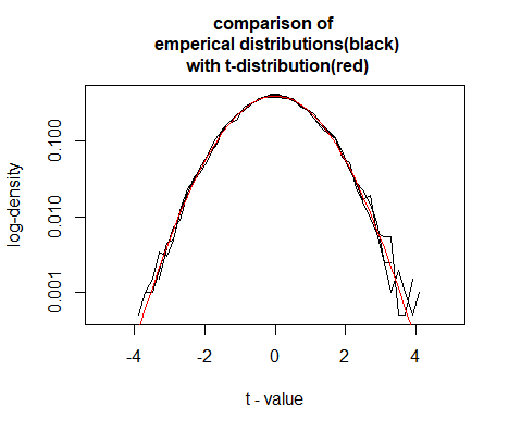
In the above image you see that there is still some reasonable difference in the distribution of $\hat\sigma$, but in the distribution of the values $t=(\bar{x}_1-\bar{x}_2)/\hat\sigma$ there is hardly any difference as you can see below.

---

So you need not worry much about using a t-test when the samples/population are not exactly normal distributed. The t-test is not very sensitive to deviations like these because with large samples the distribution of the sample mean is gonna approximate a normal distribution no matter what the underlying distribution is. And the distribution of the sample mean scaled by the sample standard deviation is gonna approximate a t-distribution/normal distribution as well because the error in the estimate of the standard deviation is gonna reduce for larger samples.

In fact: As the sample size gets larger the importance of the normality of the population distribution decreases. But, ironically the probability that a normality test displays a significant difference from a normal distribution increases (because most populations in real life are not exactly normally distributed and given large enough sample size the probability to get a significant difference increases, but 'significance' should not be given any weight, it is about the size of the difference with normality)

The exception is: 1 distribution with infinite variance or very high kurtosis such that the sample mean does not approach a normal distribution quickly. 2 when the sample size is small.

You can use simulations based on empirical distribution (or maybe you have theoretical consideration that allow you to make assumptions about the population distribution) to verify whether the approximation with a t-distribution make sense.

set.seed(1)

nt <- 10^4  # we do 10^4 trials
ns<- 50     # with samples of size 50

tm <- c()

for (j in 1:3) {
  # generate samples in a matrix
  if (j ==1) {
    x <- matrix(rnorm(nt*ns,0,10),nt)
    y <- matrix(rnorm(nt*ns,0,10),nt)
  }
  if (j == 2) {
    x <- matrix(runif(nt*ns,-sqrt(300),sqrt(300)),nt)
    y <- matrix(runif(nt*ns,-sqrt(300),sqrt(300)),nt)
  }
  if (j == 3) {
    x <- matrix(rt(nt*ns,3),nt)*sqrt(100/3)
    y <- matrix(rt(nt*ns,3),nt)*sqrt(100/3)
  }
  # compute statistics/estimates (means and pooled standard deviation)
  xm <- rowMeans(x)
  ym <- rowMeans(y)
  s_est <- sapply(1:nt, FUN = function(i) sqrt(sd(x[i,])^2 + sd(y[i,])^2)/sqrt(ns))

  # perform t-test
  t_est <- sapply(1:nt, FUN = function(i) t.test(x[i,],y[i,])$p.value)
  colours <- hsv(0,(t_est<=0.05),(t_est<=0.05),0.3)

  # display in plot
  plot(xm-ym,s_est, ylim = c(0,3), xlim = c(-10,10),
       xlab = "sample mean difference",
       ylab = "sample mean difference \n estimated standard deviation",
       col = colours, bg = colours, pch = 21, cex =0.3)
  sum((t_est<=0.05))/nt

  # the limits used by the t-test
  lines(c(0,10),c(0,10)/qt(0.975,ns*2-2))
  lines(-c(0,10),c(0,10)/qt(0.975,ns*2-2))
  tm <- rbind(tm,(xm-ym)/s_est)

  title(c("samples from normal distribution",
         "samples from uniform distribution",
         "samples from t-distribution"
         )[j],cex.main = 1)
}

h1 <- hist(tm[1,],breaks = seq(-10,10,0.2))
h2 <- hist(tm[2,],breaks = seq(-10,10,0.2))
h3 <- hist(tm[3,],breaks = seq(-10,10,0.2))
plot(h1$mids,h1$density, type = "l", xlim = c(-5,5), log = "y",
     ylab = "log-density", xlab = "t - value",
     yaxt = "n")
axis(2,at = c(0.001,0.01,0.1,1))
lines(h2$mids,h2$density)
lines(h3$mids,h3$density)
lines(h1$mids,dt(h1$mids,98), col =2)
title("comparison of \n emperical distributions(black)\n with t-distribution(red)", cex.main = 1)

About the difference with the Mann Whitney U test

In your case the Mann-Whitney U test is significant and the t-test is not, even though the Mann-Whitney U test is generally considered to have a lower power (and hence will be less likely to turn significant if there is a difference).

The reason for this might be that you are dealing with a distribution that has a few large outliers that make the estimate of the variance very large and the t statistic very low. (although as explained further below, for a given distribution you may often get different results for Mann-Whitney and t-test)

It is a bit difficult to go change things afterwards (because it is a bit cherry picking to go look for whichever test gives the result that you desire/expect). But for the next time that you perform a test and you expect that these outliers are gonna make the t-test inaccurate, then you may either use the Mann-Whitney U test or find some way to deal with outliers (maybe it makes sense to use a different scale, or the average of the samples with outliers removed). Also, maybe you should not be comparing the means of the samples, but a different statistic makes more sense (e.g. the medium or some other values). The groups may differ on more aspects than just the mean.

Keep in mind that a Mann-Whitney U test is answering a different question than the question whether two populations have the same means or not.

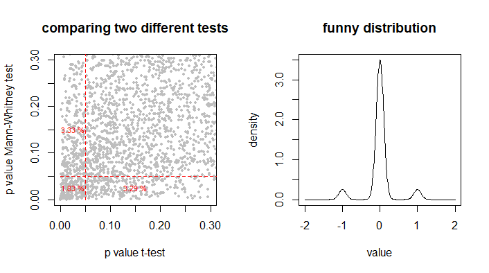
This is demonstrated in the example below. For some funny shaped population distribution (in order to make the outcome more extreme, with other types of distributions the effect will be less) we take 1000 times two samples of size 50 and compare them based 95% t-test and Mann-Whitney test. Overall, the two tests each reject about 5% of the time the null hypothesis, however they only do this at the same time only in 2% of the cases.

For this particular case it means that when you are rejecting the null hypothesis when either the Mann-Whitney or the t-test is with a p-value below 0.05, then this is not occurring in 5% of the cases, but instead in 8% of the cases. (and that is the 'problem' of cherry picking and peeking at multiple types of test instead of deciding beforehand what sort of test should be appropriate to use)

ns <- 50      # samples of size 50
nt <- 10^4    # compare 10^4 tests

# pU and pT will contain the p-values of the tests
pU <- rep(nt,0)   
pT <- rep(nt,0)

# simulate data and perform tests nt times
for (i in 1:nt) {
  # some funny distribution with three modes
  xy <- c(-1,0,0,0,1)[1+rbinom(ns,4,0.5)]
  y <- rnorm(ns,xy,0.1)
  xz <- c(-1,0,0,0,1)[1+rbinom(ns,4,0.5)]
  z <- rnorm(ns,xz,0.1)

  # perform tests
  pT[i] <- t.test(y,z)$p.value
  pU[i] <- wilcox.test(y,z)$p.value
}

# plot results of different p values
plot(pT,pU, xlim = c(0,0.3), ylim = c(0,0.3),
     xlab = "p value t-test", ylab = "p value Mann-Whitney test", 
     main = "comparing two different tests", pch = 21 , col = 8, bg = 8, cex = 0.5)

# plotting percentage of points in different regions
lines(c(0.05)*c(1,1),c(0,1), col = 2, lty = 2)
lines(c(0,1), c(0.05)*c(1,1), col = 2, lty = 2)
text(0.025,0.025, paste0(100*sum((pT <= 0.05)*(pU <= 0.05))/nt, " %"), cex = 0.7, col= 2 )
text(0.15,0.025, paste0(100*sum((pT > 0.05)*(pU <= 0.05))/nt, " %"), cex = 0.7, col= 2 )
text(0.025,0.15, paste0(100*sum((pT <= 0.05)*(pU > 0.05))/nt, " %"), cex = 0.7, col= 2 )

# plotting the shape of the population distribution
# from which the samples where drawn
t <- seq(-2,2,0.01)
plot(t,0.5^4*dnorm(t,-1,0.1)+0.5^4*dnorm(t,1,0.1)+(1-0.5^3)*dnorm(t,0,0.1), type = 'l',
     xlab = "value", ylab = "density", main = "funny distribution")