I just posted an answer here https://stats.stackexchange.com/a/483133/102879 to a similar question, so I thought I would modify it for this one.
Whether you use Stata or any other package is not relevant. Here is R code that anyone can run:
y = c(2.5,3.5,4.7, 3.2 ,4.1,5.0)
x = c(1.5,2.0,2.5,3.5,4.0, 4.3)
z = c(1,1,1,2,2,2)

summary(lm(y~x))
summary(lm(y~x+z))

plot(x,y,col=x2)
legend("topleft", c("z=1", "z=2"), pch=1, col=1:2)
In the regression of y on x, $\hat \beta_1 = 0.5233$. But in the regression of y on x and z, $\hat \beta_1 = 2.2016$.
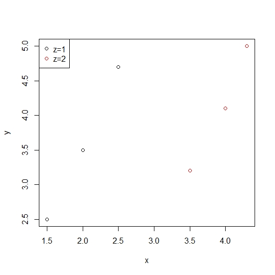
The discrepancy is easily explained by the following graph:

Ignoring the value of z, there is a weak positive trend relating y and x that can be seen in the graph, given by the least squares slope $\hat \beta_1 = 0.5233$. But within levels of z, (ie, fixing z at either 1 or 2), there is a much steeper slope relating y and x, given by $\hat \beta_1 = 2.2016$, which you can think of as kind of an average slope for the two groups. The main difference is in the "held fixed" idea: In the simple regression, z is not held fixed in the interpretation of $\beta_1$. But in the regression with both x and z, $\beta_1$ refers to the effect of x while z is held fixed (at either 1 or 2 in this example).
(A side note: one might think that the slope relating y and x should differ for the two different groups, z=1 and z=2. An assumption of the additive model is that these slopes are exactly the same. You can relax that assumption by including the interaction term z*x in the regression model; this will allow the two slopes to be estimated exactly as if the two groups were analyzed separately.)

