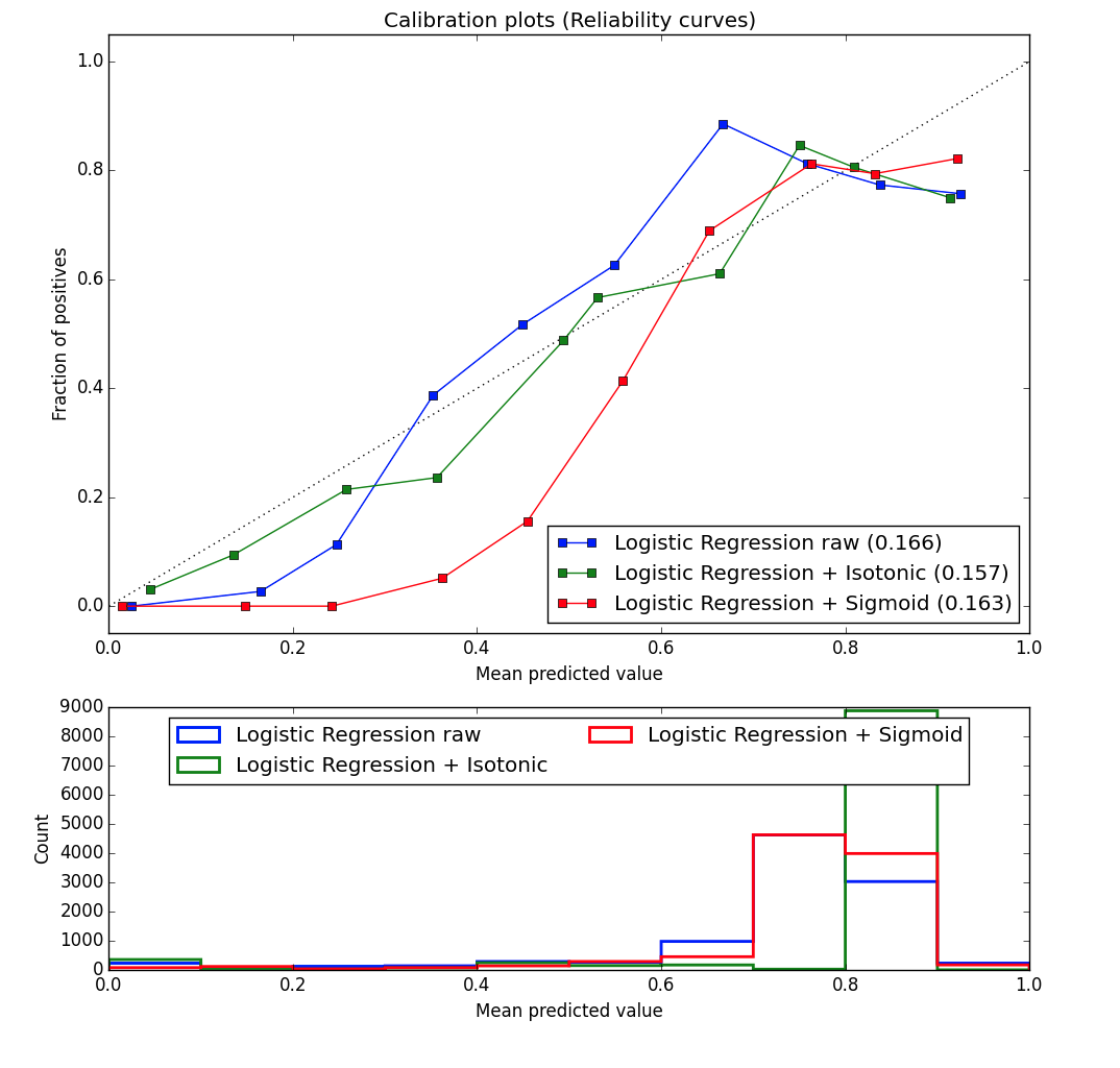
You may get discrepancies like these, decreases in the reliability curves, when the model used for fitting is not capturing the true model accurately.
For instance when you fit data that follows a quadratic relationship with a linear curve, then you will get that a plot of the residuals shows some trend of varying over/underestimating. Something similar can happen with a plot of probabilities (which is sort of a residual plot of predicted versus observed plot).
Then, we want the "fraction of positives" to be a non-decreasing function of "mean predicted values", which is done by isotonic regression.
The is isotonic regression does not relate to the reliability curve being monotonoc and increasing. It is the fitted probability value that is a monotonic increasing/decreasing function (as function of some predictor parameter).
The data and neither the residuals need to be monotonic increasing/decreasing. Also the observed as function of fitted need not to be a monotonic function.
For instance, if you have a decrease of $p$ towards the end, then monotonic regression might be overestimating those last values (because it will cause a lower error for the other values), and you will get a decrease in the plot of observed versus predicted.
(or imagine how monotonic regression would fit a sine curve)
We might illustrate this behavior with a simple example.
Say we have Bernoulli distributed data where the logit of the probability is a quadratic function of some regressor. And say that we fit this logit with a linear function instead of a quadratic function.
You can imagine that the linear curve will be differently overestimating and underestimating the probability parameter in different regions.
For the example from the code below
$$p_{true} = \text{logistic}(8+6x+x^2) = \frac{1}{1+e^{-8-6x-x^2}} $$
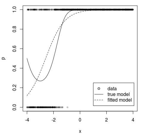
it will look like this when we sample 10k points with $-4<x<4$:

Here you see the varying pattern of over/under-estimating when we fit a quadratic curve with a straight line.
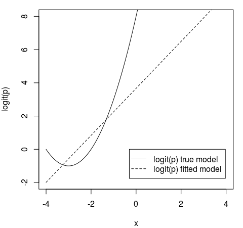
Sidenote: it doesn't look like we fit with a straight line because it is the logistic function applied to a straight line. So below we plot the logit of the probabilities and it shows the linear and quadratic curves:

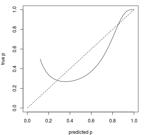
We can also plot a curve of the predicted versus the true probability parameter.

The plot above is not the same as yours, it is not binned data, but it does show that the curve can be decreasing and does not need to be non-decreasing.
In the case with binned observed data, which is stochastic, you may get additional variations/noise, which can cause the curve to be non-decreasing.
### logistic function
flogistic <- function(x) {
  1/(1+exp(-x))
}

### generate bernoulli distributed data
### the probability is modeled with a QUADRATIC funcion
set.seed(1)
x <- runif(10^3,-4,4)
p <- flogistic((x+4)*(x+2))
y <- rbinom(10^3,size = 1, prob=p)

### fit with LINEAR function
mod <- glm(y~x, family = binomial(link = "logit"))
mod

### plotting observations
xs <- seq(-4,4,0.001)
plot(x,y, pch = 21, col = rgb(0,0,0,0.2), bg = rgb(0,0,0,0.2), cex = 0.7, ylab = "p" )
### this is the true model
lines(xs,flogistic((xs+4)*(xs+2)))
### this is the fitted model
lines(xs,flogistic(mod$coefficients[1]+mod$coefficients[2]*xs), lty = 2)
legend(-4,0.9, c("data","true model", "fitted model"),
       lty = c(NA,1,2), pch = c(21,NA,NA), col = 1, pt.bg=rgb(0,0,0,0.2))

### plotting logit
xs <- seq(-4,4,0.001)
plot(-100,-100, pch = 21, col = rgb(0,0,0,0.2), bg = rgb(0,0,0,0.2), cex = 0.7,
     xlim = c(-4,4), ylim = c(-4,4), xlab = "x", ylab = "logit(p)")
### this is the true model
lines(xs,(xs+4)*(xs+2))
### this is the fitted model
lines(xs,(mod$coefficients[1]+mod$coefficients[2]*xs), lty = 2)
legend(-4,4, c("logit(p) true model", "logit(p) fitted model"),
       lty = c(1,2), pch = c(NA,NA), col = 1, pt.bg=rgb(0,0,0,0.2))

###
plot(flogistic(mod$coefficients[1]+mod$coefficients[2]*xs),flogistic((xs+4)*(xs+2)),
     type = "l", xlab = "predicted p", ylab = "true p",
     xlim = c(0,1),ylim=c(0,1))
lines(c(0,1),c(0,1), lty = 2)

