Why don't I see a minimum in out-of-sample mean squared error along my lasso path?

Question

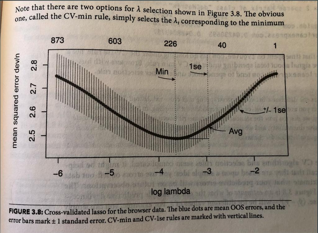
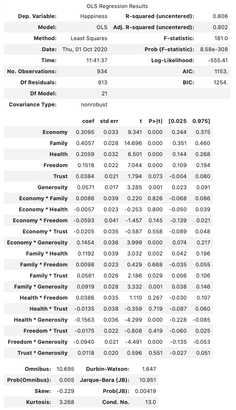
I'm hoping to reproduce the following figure from Matt Taddy's book Business Data Science using the Happiness data set from Kaggle.

Running linear regression using lasso regularization, he observes a minimum in the out-of-sample (OOS) mean squared error and asserts that this value of lambda represents a good choice for regularization. Makes sense.

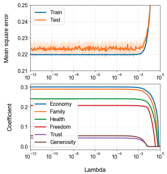
When I try the same thing on the happiness data set, a couple things look right: in-sample MSE is lower than out-of-sample MSE, and coefficients go to zero as regularization parameter is increased.

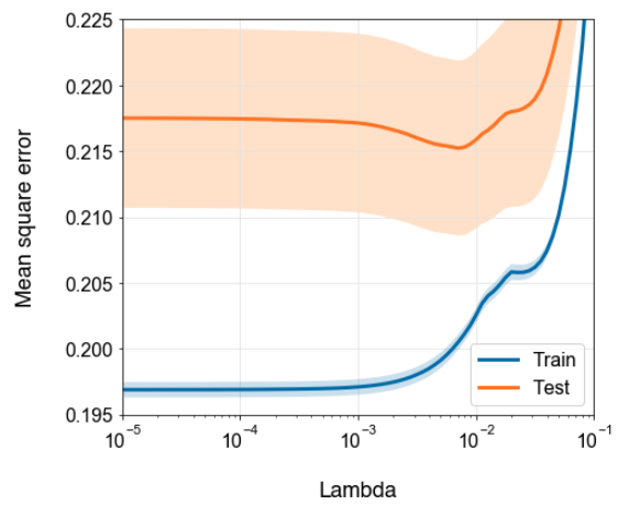
However, I don't see any drop in out-of-sample mean squared error with increasing lambda -- it's noisy and flat (top plot, orange trace).

As I understand it, dialing up lambda (sklearn.linear_model.Lasso() calls this alpha) should reduce OOS MSE as the fitted coefficients generalize better to the unseen data.

Why might I not be seeing a minimum in OOS MSE?

I wrote up the code myself because I wanted to understand how it works. I used 10-fold cross-validation with shuffled sampling and scanned 300 points across the regularization range of 10^-12 <= alpha <= 1.

Here it is:

# k-fold cross validation with lasso regularization
import numpy as np
alphas = np.logspace(-12, 0, 301)

coefs_all = []
coefs_avg_all = []
coefs_std_all = []
mse_train_avg_all = []
mse_test_avg_all = []
mse_train_std_all = []
mse_test_std_all = []

for alpha in alphas:

    # randomly split data into k folds
    from sklearn.model_selection import KFold
    folds = 10
    kf = KFold(n_splits=folds, shuffle=True)

    coefs = []
    mse_train = []
    mse_test = []
    
    for train_index, test_index in kf.split(X):
        X_train, X_test = X.iloc[train_index], X.iloc[test_index]
        y_train, y_test = y.iloc[train_index], y.iloc[test_index]

        # build model on training data and get coefficients
        from sklearn import linear_model
        lasso = linear_model.Lasso(alpha=alpha)
        lasso.fit(X_train, y_train)
        coefs_fold = lasso.coef_
        
        # get mean squared error of model predictions
        y_pred_train_fold = np.dot(X_train, coefs_fold)
        y_pred_test_fold = np.dot(X_test, coefs_fold)
        mse_train_fold = sum((y_train - y_pred_train_fold) ** 2) / len(y_train)
        mse_test_fold = sum((y_test - y_pred_test_fold) ** 2) / len(y_test) 
        
        # for each fold, add coeffs and mses to growing list
        coefs.append(coefs_fold)
        mse_train.append(mse_train_fold)
        mse_test.append(mse_test_fold)

    # across folds at this alpha, get average values of coefficients, mses, and stdevs
    coefs_avg_alpha = [sum(items) / len(coefs) for items in zip(*coefs)]
    coefs_std_alpha = [np.std(items) for items in zip(*coefs)]
    mse_train_avg_alpha = np.average(mse_train)
    mse_test_avg_alpha = np.average(mse_test)
    mse_train_std_alpha = np.std(mse_train)
    mse_test_std_alpha = np.std(mse_test)

    # compile these average values into growing list
    coefs_avg_all.append(coefs_avg_alpha)
    coefs_std_all.append(coefs_std_alpha)
    mse_train_avg_all.append(mse_train_avg_alpha)
    mse_test_avg_all.append(mse_test_avg_alpha)
    mse_train_std_all.append(mse_train_std_alpha)
    mse_test_std_all.append(mse_test_std_alpha)
    
# compile mean square error summary into dataframe
mse_df = pd.DataFrame({'Alpha': alphas,
                       'MSE train avg': mse_train_avg_all,
                       'MSE test avg': mse_test_avg_all,
                       'MSE train std': mse_train_std_all,
                       'MSE test std': mse_test_std_all})

# bind coefficients to previous dataframe
coefs_df = pd.DataFrame(coefs_avg_all, columns=X.columns.to_list())
lasso_cv_summary_df = pd.concat([mse_df, coefs_df], axis=1)

Answer 1

A minimum in out-of-sample mean squared error (OOS MSE) is found only when the unregularized model is prone to overfitting.

The simple model for the happiness response variable using only the 6 features provided is on the high-bias side of the bias-variance tradeoff. It's not possible to overfit the data using a linear model here.

Expanding the feature space by adding interaction terms, for example, allows for the possibility of overfitting. In this case, the lasso path does indeed show a minimum in OOS MSE:

Consider the unregularized models:

6 features -- all features are significant at 95% confidence (P-values << 0.05):

21 features (6 + 15 interaction terms) -- several of the new terms merely add noise (P-values > 0.05):