What are reasonable ways to plot the "pdf" of a censored random variable?

Question

Objective: Just to help close a hole in my statistical knowledge (as opposed to having a practical subject matter need), I want to know what are some of the ways to display what I am calling a probability density function when the probability density function does not exist for one or more values of the random variable.

However, maybe the presumption that one can do this in the first place should be answered first. Yes, the cumulative distribution function can be plotted. And the derivative of that function for the example below exists for all points but one.

But if the derivative doesn't exist for a single point, does that mean the pdf doesn't exist for the random variable? If so, can I get around that by simply saying I have a "quasi-pdf" ? I find it hard to believe this isn't legitimate. But I've been wrong many times before. Maybe this is just a big hole in my knowledge of random variables.

Example:

Suppose $X \sim N (\mu, \sigma^2) $ and that $Y = \max (0, X) $. The CDF of $Y$ is

$$\begin{eqnarray*} \text{Pr}(Y \leq y) & = & 0 \quad \quad \quad \quad \quad \enspace \text{for } y<0 \notag \\ & = & \Phi\left((y-\mu)/\sigma\right) \text{ for } y\geq 0 \notag \\ \end{eqnarray*}$$

where $\Phi()$ is the standard normal cumulative distribution function.

What are reasonable ways to plot the "PDF" (the derivative of the CDF) when the PDF does not exist at $Y=0$? (A subquestion is "should" one attempt such a plot. I say absolutely "Yes" while at least one other says "No".)

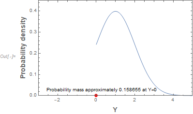
Here is one way simply using a "dot" at the point (0,0) and a text explanation in the figure:

Are there standard/reasonable ways to do this which might include something (a circle or rectangle) proportional to the size of the probability mass?

This is related to a comment I made (and the associated discussion) on Mathematica StackExchange.

Answer 1

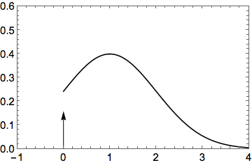
If your main objective is to understand what's going on with these mixed continuous-and-discrete "pdfs," then you might want to consider learning some measure theory. The article that @angryavian shared in the comments is probably a sufficient answer to your stated question about plotting these, but you might want to consider using the graphical representation of a Dirac delta (generalized) function instead (an arrow) instead of the line-point representation that the article uses. While strictly speaking, the probability density function (pdf) does not exist in your example, you can consider the "pdf" to be the generalized function (Schwarz distribution) given by $$ f(x) = \delta(x)\int_{-\infty}^0 \mathcal{N}(\mu, \sigma^2)(x) dx + I_{[0,\infty)}(x) \mathcal{N}(\mu, \sigma^2)(x) $$ where $\mathcal{N}(\mu, \sigma^2)$ is the normal distribution pdf, $I_{[0,\infty)}$ is the indicator function for the set $[0,\infty)$, and $\delta$ is the Dirac delta (generalized) function. This generalized function $f$ can be used as a "pdf" in the same way you would use a true pdf because $$ \int_A f(x)dx = P(A) \text{ for all measurable sets } A \subset \mathbb{R}. $$ And using the arrow representation of a Dirac delta, you can graph $f$ as: