spatstat::plot.envelope observed line longer than shading

Question

Using the R package spatstat I'm plotting pooled pointwise envelopes of the function Jfox calculated for different point pattern in an hyperframe.

The workflow is as follow:

# define distances to make envelopes comparables
ers<-seq(from=0,to=3, by=0.01) 

# calculate the envelopes for the Jfox function for each point pattern in an hyperframe
urc_hyp$env_Jfox<-with(urc_hyp, envelope(Y=urc_ppp,  fun=Jfox, funargs=list(Y=pref_im), r=ers,nsim=39, fix.n=T,savefuns=TRUE, global=FALSE, nrank=1, correction='best', eps=0.1)

# split the hyperframe according to a factor
env_split<-split(urc_hyp$env_Jfox, urc_hyp$matrix)
# pool the envelopes for patterns splitted by factor
env_pool <- anylapply(env_split, FUN= pool)

You can find the env_pool object here. I can see that each envelope has an attribute of suggested (r) values:

env_pool[[1]]

Pointwise critical envelopes for J[fox](r)
and observed value for ‘urc_ppp’
Obtained from 78 simulations of CSR with fixed number of points
Alternative: two.sided
Significance level of pointwise Monte Carlo test: 2/79 = 0.0253
..................................................................................
     Math.label             Description                                           
r    r                      distance argument r                                   
obs  {hat(J)[fox]^{obs}}(r) observed value of J[fox](r) for data pattern          
theo {J[fox]^{theo}}(r)     theoretical value of J[fox](r) for CSR                
lo   {hat(J)[fox]^{lo}}(r)  lower pointwise envelope of J[fox](r) from simulations
hi   {hat(J)[fox]^{hi}}(r)  upper pointwise envelope of J[fox](r) from simulations
..................................................................................
Default plot formula:  .~r
where “.” stands for ‘obs’, ‘theo’, ‘hi’, ‘lo’
Columns ‘lo’ and ‘hi’ will be plotted as shading (by default)
Recommended range of argument r: [0, 0.46]
Available range of argument r: [0, 3]

So here, for example, the recomended rance goes from 0 to 0.46, while the available range is up to 3 (which is the limit I set to all the envelopes to make them comprable).

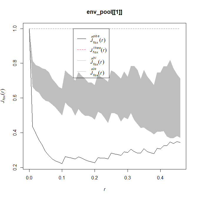
Now if I plot without specifying the range of the x axis, the plot function use by default the recomended range:

 plot(env_pool[[1]])

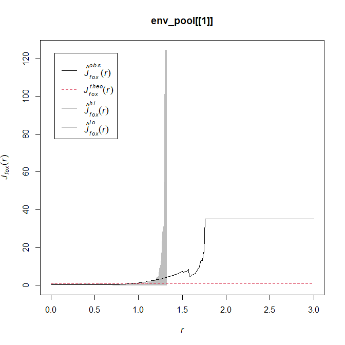
but If I specify the xlim I get this:

 plot(env_pool[[1]], xlim=c(0,3) )

Now, in the last figure you can see that the shaded area (which represents the significant band, as per ?envelope) extend beyond the recomended range for r.

However the shading does not extend to the whole length of the black line (i.e. the observed JFox curve).

In some case the shading falls short even within the recommended r range (e.g. plot(env_pool[[2]])

Is there theoretical a reason for this and if so how should I interpret the line after the shading?

Or is it due to some plotting parameter that should be modified/specified?

Answer 1

This behaviour is correct. The shaded region is the envelope of 39 curves which were each computed by generating a completely random pattern and computing the estimate of Foxall's J function Jfox for the pattern. The J functions are ratios of survival functions, J(r) = (1-G(r))/(1-F(r)) where F and G are estimates of the cumulative distribution functions of certain distances in the point pattern. The estimate of J(r) is obviously undefined if the estimate of F(r) is zero. When that happens, the estimate of J(r) is returned by Jfox as NA or NaN. The envelope function discards any such values when determining the envelope. A value of NA or NaN in the envelope at a certain value of r means that all of the simulated J function values were NA or NaN. That is, out of 39 random point patterns, none of the point patterns had an empty-space distance greater than this distance r. The data point pattern is different from the random patterns in that it apparently has some very large empty-space distances.

Answer 2

I'm on my phone so can't check any details, but my best guess is that the upper bound of the envelope (hi) is NA when the shading stops. You can use as.data.frame to convert the envelope to a data.frame and inspect the values. This may be a mathematical problem with the estimator and not a computational problem / bug, but I can't investigate right now.