pointwise envelopes not including Theoretical line Foxall J

Question

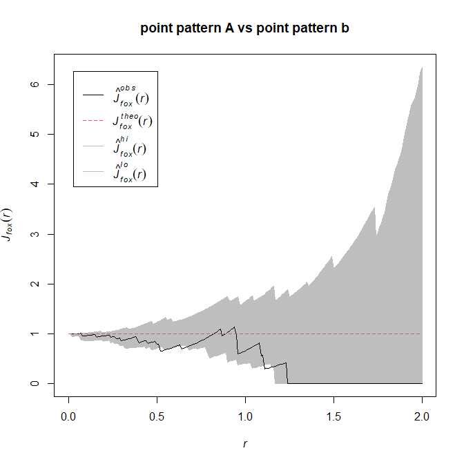
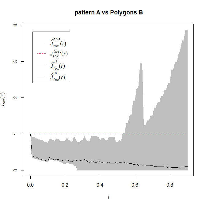
I am computing pointwise envelopes for the Foxall's J function to investigate the whether some point patterns of interest are clustered, avoid or are independent from other point patterns or polygons.

I am doing this using spatstat with a syntax similar to this (reproducible example provided below):

evelope(my_pattern_of_interest, fun=Jfox, funargs=list(Y=my_other_patten),...)

I am calculating the envelopes for several replicated patterns (i.e., different transects) and then plotting the pooled (i.e., pool) envelopes.

So far, whenever the Jfox is calculated between 2 point patterns, the shaded area representing the simulation envelope includes the theoretical line (i.e., represented by red dashes), as in this example:

Figure 1

Instead, when Jfox is calculated between a point pattern and polygons, it is frequent that the envelope area does not include the Theroretical line (at least in some regions). Like in this example:

Figure 2

What does this means?

From my understanding so far, if - or rather "where" since these are pointwise envelopes - the observed line (solid black) is within the shaded area, it means that the observed pattern (say clustering as in Figure 2) is not significantly different from what could be observed at random. Alternatively, if/where the observed line is out of the shaded area, then I have a significant difference.

What does the fact that the theoretical line lays outside the shaded area mean? Is it giving me another piece of information? How should I interpret this?

Reproducible example

Download the hyperframe for the example from here.

# Load the hyperframe 
# --------------------

# The hyperframe contains the ppp and IM mask (for polygons) used in this example.
# Variable 'trs' is the identity of replicated point patter (i.e. a transect). Unit measure is 'meter'.
# For the sake of speed, the hyperframe already contains also the evelopes for each replicated pattern, but the code used to produce them is below.

load('Q575569-envelopes-hyperframe.Rdata')

# Compute the envelopes 
# -----------------------

# define distances to make envelopes comparables
EPS=0.1
ers<-seq(0, 3, 0.01)
nsims<-6

# Envelopes (since this may take some time, you may skip this and find the envelopes already included in the hyperframe)
hypCV$lept_arub_jfoxPTW<-with(hypCV,
                            envelope(Y=lept, fun=Jfox, funargs=list(Y=arub), r=ers, nsim=nsims, fix.n=T, savefuns=T, global=F, nrank=1, correction='best', eps=EPS) )


# ppp A vs polygons (in reality a mask as a proxy for polygons)  
hypCV$arub_LSsubs_jfoxPTW<-with(hypCV,
                            envelope(Y=arub, fun=Jfox, funargs=list(Y=rkaIM), r=ers, nsim=nsims, fix.n=T, savefuns=T, global=F, nrank=1, correction='best', eps=EPS) )

#  Pool and plot
# ------------------

# pooling all transects together.
AB<-pool(hypCV$lept_arub_jfoxPTW)
APoly<-pool(hypCV$arub_LSsubs_jfoxPTW)

# plot
par(mfrow=c(1,2))
plot(AB, main='ppp A vs ppp B', xlim=c(0,2))
plot(APoly, main='ppp A vs poly', legendpos='topleft', xlim=c(0,1))

Thank you.

Answer 1

Please provide a minimal working example.

Pooling of objects (such as simulation envelopes) is only justified when the individual objects (envelopes) were created under identical conditions. In your example you appear to be pooling several envelopes of the Foxall J function Jfox(X,Y) that were computed for different datasets. Each envelope was computed by taking a particular dataset (X,Y), holding Y fixed, and generating random point patterns Xsim with the same average intensity as X. These are not identical conditions between the different envelopes, so it is not valid to pool them, and paradoxes can occur, such as you have found.

Again, a minimal working example would help.