$R^2$ on out-sample data set

Question

The conventional definition of $R^2$ is: $R^2 = 1-SSE/SST$, where SSE denotes sum of squared errors and SST is total sum of squares ($n\times variance$, n being number of sample points in train set).

However, I want to see the fitness of my model on out-of-sample set (test set) or both train and test sets combined. Is it fine to use the same definition of $R^2$ by taking SSE and SST appropriately over test set or (train+test) sets, respectively? Eg. I train my model on $n$ sample points. I want to check its performance on ($n+p$) points ($p$ being some new sample points out of the train set). Can I use $R^2 = 1-(SSE$ on (n+p) points$)/(SST$ on (n+p) points$)$?

Answer 1

There are several definitions of $R^2$ that are equivalent for in-sample OLS linear regression.

1. The squared correlation between the $x$ and $y$ in simple linear regression

2. The squared correlation between the predictions $\hat y$ and truth $y$

3. The proportion of variance explained

4. A comparison of the model performance to the performance of a naïve model that always predicts $\bar y$, no matter what values the features take

The final one is the one that makes the most sense to me.

When you get to out-of-sample $R^2$, the first three present issues.

1. Typically, an out-of-sample metric is of interest to problems that require more complicated feature spaces than just one variable, so this is out.

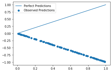
2. Out-of-sample, all bets are off. If you've badly overfit, you could be in a position where high values of $y$ correspond to low values of $\hat y$, and low values of $y$ correspond to high values of $\hat y$, the extreme of which is $\hat y = -y$. This puts you in a position where $cor(y, \hat y)<0$, and when you square that value, you miss that the predictions are terrible. Further, this approach misses systematic bias (consistently predicting too high or too low by $k$) and predicting multiples of the true values. That is, if $\hat y = a+b y$ for $(a,b)\ne(0,1)$, $cor(y, \hat y)$ is oblivious to the poor predictions. That this metric misses such critical information is, to me, a dealbreaker.

3. This one is appealing, but the "proportion of variance explained" interpretation of $R^2$ breaks down in most situations. Out-of-sample is one such situation, as the coefficients that result in the orthogonality needed for this interpretation to hold out-of-sample are unlikely to be the coefficients estimated in-sample, even for an OLS linear regression.

4. Finally, this one makes sense. We have a model and are interested in the square loss. As minimizing square loss corresponds to finding the conditional mean, a good benchmark is to see if the predictions are better than a model that always predicts the conditional mean to be the pooled mean.

$$ \dfrac{ \sum_{i=1}^n\big( y_i - \hat y_i \big)^2 }{ \sum_{i=1}^n\big( y_i - \bar y \big)^2 } $$

If the numerator is smaller than the denominator, it means that our predictions beat the predictions made by out baseline model that naïvely predicts $\bar y$ every time. If the numerator is larger than the denominator, then all of our statistics and machine learning efforts are doing worse than we would do by predicting AVERAGE(A:A) (to use some Excel terminology). That is, our model is doing a poor job of predicting.

It is typical to subtract this quantity from $1$ in order to align with the other three ways of defining in-sample $R^2$.

$$R^2 = 1- \dfrac{ \sum_{i=1}^n\big( y_i - \hat y_i \big)^2 }{ \sum_{i=1}^n\big( y_i - \bar y \big)^2 } $$

This idea of comparing to a baseline model exists for other metrics. For logistic regressions, there are two named metrics that do exactly this: Efron's and McFadden's pseudo $R^2$, as discussed on this UCLA page.

For evaluating an out-of-sample $R^2$, I would use the following:

$$R^2_{oos}=1- \dfrac{ \sum_{i=1}^n\big( y_i - \hat y_i \big)^2 }{ \sum_{i=1}^n\big( y_i - \bar y_{train} \big)^2 } $$

This compares the out-of-sample performance of your model to the out-of-sample performance you would get from a model trained just to predict the mean every time (the naïve baseline model).

Irritatingly, the popular Python machine learning package sklearn has an out-of-sample $R^2$ function, sklearn.metrics.r2_score, that uses the $\bar y$ from whatever you input as the truth values. This is fine for in-sample $R^2$, but for out-of-sample $R^2$, it results in the following formula:

$$R^2_{oos}1- \dfrac{ \sum_{i=1}^n\big( y_i - \hat y_i \big)^2 }{ \sum_{i=1}^n\big( y_i - \bar y_{test} \big)^2 } $$

The denominator is now based on the square loss of an intercept-only linear model that has been trained on the test data. We should never have access to this model, as it requires us to train on the test data, and I disagree with the sklearn implementation. Fortunately, however, this function does not fall for the traps that just the $cor(y, \hat y)$ does.

np.random.seed(2022)

N = 100
y = np.random.uniform(0, 1, N)

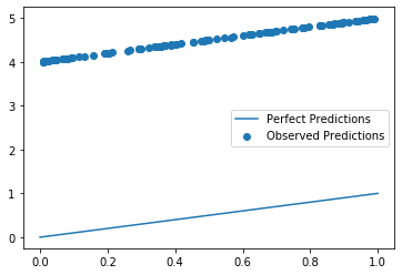
yhat1 = y + 4
plt.scatter(y, yhat1, label = "Observed Predictions")
plt.plot([0, 1], [0, 1], label = "Perfect Predictions")
plt.legend()
plt.show()
plt.close()
print("sklearn R^2: ", r2_score(y, yhat1))
print("Squared correlation between observations and predictions: ", np.corrcoef(y, yhat1)[1, 1]**2)

sklearn R^2: -157.49362110734847

Squared correlation between observations and predictions: 1.0

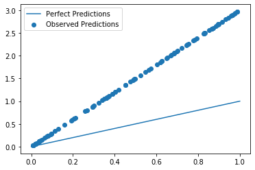
yhat2 = y * 3
plt.scatter(y, yhat2, label = "Observed Predictions")
plt.plot([0, 1], [0, 1], label = "Perfect Predictions")
plt.legend()
plt.show()
plt.close()
print("sklearn R^2: ", r2_score(y, yhat2))
print("Squared correlation between observations and predictions: ", np.corrcoef(y, yhat2)[1, 1]**2)

sklearn R^2: -12.341142004503533

Squared correlation between observations and predictions: 1.0

yhat3 = -y
plt.scatter(y, yhat3, label = "Observed Predictions")
plt.plot([0, 1], [0, 1], label = "Perfect Predictions")
plt.legend()
plt.show()
plt.close()
print("sklearn R^2: ", r2_score(y, yhat3))
print("Squared correlation between observations and predictions: ", np.corrcoef(y, yhat3)[1, 1]**2)

sklearn R^2: -12.341142004503533

Squared correlation between observations and predictions: 1.0

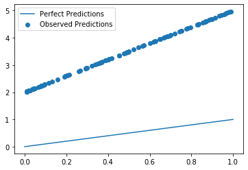
yhat4 = 2 + 3*y
plt.scatter(y, yhat4, label = "Observed Predictions")
plt.plot([0, 1], [0, 1], label = "Perfect Predictions")
plt.legend()
plt.show()
plt.close()
print("sklearn R^2: ", r2_score(y, yhat4))
print("Squared correlation between observations and predictions: ", np.corrcoef(y, yhat4)[1, 1]**2)

sklearn R^2: -90.44196171593748

Squared correlation between observations and predictions: 1.0

In all of these situations, the squared correlation between the predictions and the truth is a perfect-looking $1$, yet the sklearn.metrics.r2_score correctly indicates that the predictions are terrible, as is evident in all four plots.

Finally, for evaluating $R^2$ on the combined data (training and testing), it is unclear what this would tell you. If I had to do that calculation, I would be inclined to use the in-sample $\bar y$ in the denominator and just do the sums over all $n+p$ values. You might also be interested in bootstrap validation that uses all of the observations.

Answer 2

It makes sense. It is more common however to keep the training and test sets separated. So that you train your model on the train set, and then predict on the test set alone. From there you can calculate the prediction error, and a $R^2_{pred}$ if you like. (train on $n$ data points, evaluate on $p$ data points, in your terms.)

You can also look up stuff like the PRESS statistic, and other cross validation methods.

Answer 3

It makes sense to apply $R^2= 1-{\sum(y_i-\hat y_i)^2}/{\sum(y_i-\bar y)^2}$ to test set directly. It's a measure of the size of squared residuals compared to the variance of true values.

Alternatively, if you adopt the notion of deviance (see this answer), then you might use the null model from training data instead:

$$\tilde R^2= 1-\frac{\sum(y_i-\hat y_i)^2}{\sum(y_i-\bar y_{train})^2}$$

I've seen both in use, and both can be justified.