Evaluating Functional Form in Cox Regression using rcs

Question

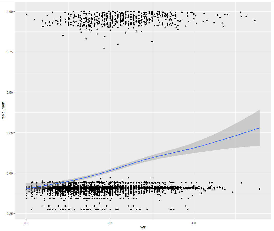
I was approaching Cox regression and need to evaluate whether is more suitable to model my independent variable as a non-linear prediction of the outcome.

Main questions is:

1. How do I check whether or not my independent variable should be modelled in a non-linear fashion?

I came into several methods, one of which was to plot the variable versus the martingale-based residual of the Cox regression (See for example www.sthda.com/english/wiki/cox-model-assumptions, last figures).

I therefore produce this type of plot with the following code, being var my independent variable:

time <- data$time 
status <- data$status 
S <- Surv(time, status) 
model1 <- coxph(S~1, data = data)
data$residual <- residuals(model1, type = "martingale")
ggplot(data = data, mapping = aes(x = var, y = residual)) +
  geom_point() +
  geom_smooth()

Here is the result:

Here comes the other questions:

2. As you can see, in my plot martingale-based residuals seems to be a lot "clustered" at extreme values, different from other plots that I found online in which residuals were more or less "uniform". I don't know how to interpret this data - seems like the data are "splitted".
3. Based on the plot, should I assume a linear relationship? I was considering to use a restricted cubic spline with 4 knots, since my guess was that a non-linear relationship may be the case here.
4. What is the correct interpretation of this plot? Do anyone have a guidance paper to interpret this plots and/or more generally speaking a guide to Cox diagnostics?

[EDIT]

This is the result of the model and of the anova as requested by @EdM - actually to generate this result I have fitted model2 with cph.

Model:

      Coef    S.E.    Wald Z Pr(>|Z|)
 var    4.5077  1.5089  2.99  0.0028  
 var'  -0.1702  4.8386 -0.04  0.9719  
 var'' -5.4636 12.5472 -0.44  0.6632 

Anova:

                    Wald Statistics          Response: S 

 Factor     Chi-Square d.f. P     
 var        217.03     3    <.0001
  Nonlinear  17.17     2    2e-04 
 TOTAL      217.03     3    <.0001

Answer 1

Instead of trying to guess from the shape of the plot of null-model martingale residuals against the value of your continuous predictor, why not let the regression itself tell you whether non-linear terms are necessary?

Harrell discusses restricted cubic splines in Section 2.4.5 of his class notes. If you fit with a restricted cubic spline, you get a set of associated coefficients, with the first being for the linear term and the rest being the coefficients of the non-linear terms. A joint test of the hypothesis that all of the non-linear term coefficients equal 0 is the test you need. See the end of that Section of the notes. If you use the rms package and its cph() command for Cox regressions, the anova() function applied to the cph object includes that test.

This regression approach has the advantage that you can apply it while taking other predictors into account. I can't say exactly why you have that particular distribution of residuals, but it might be due to other outcome-associated predictors that aren't accounted for in the null model used to generate the plot. See this answer and its link.

In response to comments and edited question:

The anova() results after modeling with the rcs() term suggest a weak overall non-linear association, dominated by the strong linear term (coefficient for var in the model results). That's consistent with the overall shape of the smoothed plot of martingale residuals.

Even though neither of the nonlinear coefficients (for var' or var") is individually distinguishable from 0 based on its own standard error, the multi-parameter Wald test used by anova() in this context also takes into account the covariance between the two coefficient estimates for non-linear terms. There's probably a very strong negative covariance between those estimates, leading to evidence that the two non-linear coefficients together have a "statistically significant" (p = 0.0002) association with outcome.

Whether that's sufficiently important in practice to devote the 2 extra degrees of freedom to non-linear modeling of var is up to you, based on your understanding of the subject matter and of your audience. With a large study like this I see no harm in keeping the non-linear terms, unless you have many other predictors to include in the model. The simple linear association might, nevertheless, be easier to explain. See Harrell's class notes, linked above, for further guidance.

Thoughts on the appearance of the martingale residual plot

Unlike some other residual types, martingale residuals are calculated for all cases, not just for cases with events. They are effectively the differences between observed and predicted event numbers for the cases. This means:

1. Martingale residuals for censored cases are necessarily negative (fewer "observed events" than predicted), so censoring patterns can influence what you see.

2. They add up overall to 0, setting constraints on the overall distribution of values (in part determined by the censored cases).

3. A null model like yours only "predicts" a combined survival curve, so you might find "extreme" residuals like this when there are many censored cases.

4. Some martingale residual plots in the literature and on line are based on multiple-regression models that include many predictors, with just one predictor of interest removed to try to gauge its functional form. As those models do a lot more "predicting" than a null model, you might find a more "uniform" distribution of residuals in those situations, when there is censoring.