Data Science Interview FAANG 2021 Question

Question

You have four tests that benchmark how much power we expect to draw from the servers in a rack: A (5 minutes), B (10 minutes), C (15 minutes) and D (30 minutes) that are conducted sequentially over the course of an hour on 10 servers in a rack. The test are run in random order on each server and all 10 server initiate the benchmark test at the same time. What is the probability that test B is running at any given time on at least 50% of the servers?

Answer 1

Let's interpret the question as asking "At any given time $t,$ what is the chance that $k=5$ or more out of $n=10$ servers are running Task B?" This interpretation is interesting due to the strange-looking behavior of the answer: there are times at which it's impossible (or highly improbable) to find many servers running Task B and other times at which it is much more likely to find many servers running Task B.

The solution is straightforward to obtain, albeit potentially terrible to compute, because the general solution requires time proportional to the number of permutations of the tasks. (Any speedup would require exploiting the summation relationships among the times; namely $5+10=15$ and $5+10+15=30.$)

In general, order the task times into an array $d=(d_1,d_2, \ldots, d_m)$ where $m$ is the number of tasks and "Task B" is indexed at position $1.$ First consider any specific server. The chance that Task B is running at time $t$ is the chance that this task began in the interval of times $(t-d_1, t].$ Suppose Task B was $k^\text{th}$ in the order, so that $k-1\ge 0$ tasks preceded it and ran to completion. Let those task indexes be the subset $S\subset \{2,3,\ldots, m\}$ and define

$$d(S) = \sum_{i\in S} d_i$$

to represent the total time taken by those tasks. We have to count the number of permutations $\sigma$ of $\{1,2,\ldots, m\}$ for which $d(\{\sigma(1),\sigma(2),\ldots,\sigma(k-1)\}\}\in (t-d_1,t]$ and $\sigma(k) = 1.$ When the $d_i$ are arbitrary durations, potentially there are as many distinct values of these $d(S)$ as there are permutations of $\{2,3,\ldots, m\}$ and $m$ cases have to be considered (for $k=1,2,\ldots, m).$ Thus the computing time cannot, in general, be reduced below $m!.$

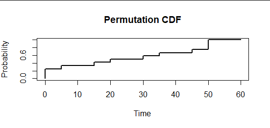
It remains only to find a reasonably clear, efficient, and correct implementation of this calculation. One way is to generate all $(m-1)!$ of the permutations of the remaining tasks $\{2,3,\ldots, m\}.$ For each such permutation $\sigma$ find the cumulative sums of the sequence $0, d_{\sigma(2)}, d_{\sigma(3)}, \ldots, d_{\sigma(m)}.$ The value of their empirical cumulative distribution function, $F,$ at time $t$ gives the chance that a randomly chosen ordered subset of the remaining tasks will be completed by time $t$ before "Task B" is run. Let's call this the "permutation ECDF." The relevant part of its graph for the data in the question looks like this:

Thus (because time is continuous), the chance that Task B is running at time $t$ must be $F(t) - F(t-d_1).$

Here is an R implementation. Given an array of times times and the index of "Task B," it returns the permutation CDF (as a function):

p.F <- function(times, index=1) {
  # Standardize the input
  d <- times
  if(isTRUE(index != 1) && isTRUE(length(d) > 1)) d[c(1, index)] <- d[c(index, 1)]
  
  # Return the CDF
  require(e1071) # Exports `permutations` to create an array of all permutations
  ecdf(apply(cbind(0, matrix(d[permutations(length(d) - 1) + 1], ncol=length(d)-1)), 1, cumsum))
}

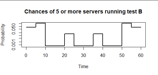
Assuming the tasks are independently ordered in each server, this chance defines a Bernoulli$(F(t)-F(t-d_1))$ distribution. Any questions about how many servers are running "Task B" at time $t$ can therefore be answered in terms of the Binomial$(n, F(t)-F(t-d_1))$ distribution. Here is a plot of those chances for the specifics of the question (on a log probability axis):

It is the graph of this R function g determined by k (equal to 5 servers), d (equal to 10 minutes), and n.servers (equal to 10 servers):

g <- function(x) pbinom(k-1, n.servers, f(x) - f(x-d), lower.tail = FALSE)

For instance, the expression g(23) returns $0.01546197$ for the chance at least $5$ of the $10$ servers are running Task B when the time is $t=23$ minutes.

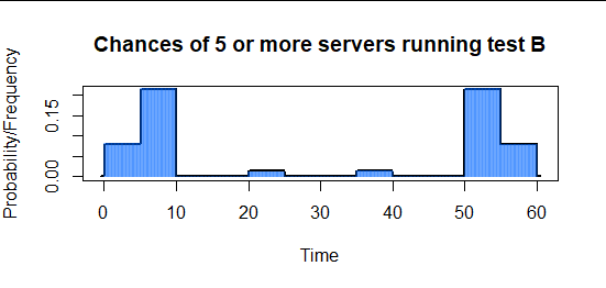
I checked this by simulating the experiment 10,000 times, in each iteration noting at which times on a fine grid "Task B" was running on five or more of the servers. The next figure plots those results in blue over the preceding chart (shown now on a linear probability scale). The agreement is good:

The structure of these plots is curious, but a little thought suggests the huge variations in probabilities are correct: after all, for half or more of the servers to be running a ten-minute task at a given intermediate time, there aren't many combinations of the remaining task times that would permit that: the occurrence of one or more of the longer tasks makes it almost impossible for this ten-minute task to be running then. And since the entire problem is the same when time is run backwards, these graphs must be symmetrical.

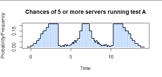
To see what the situation might look like without such a nice discretization of task times (into multiples of five minutes in the present case), here are the results (theoretical and simulated) for five randomly generated times of lengths $d=(3.4, 0.7, 0.3, 4.2, 3.9, 1.2)$ (so that "Task B" lasts 3.4 minutes).

Answer 2

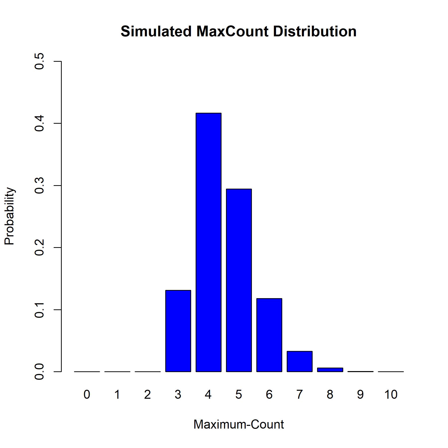
This is quite an interesting question, since it involves probability pertaining to overlapping random sets. I'm going to solve this for a more general problem where we have $K$ servers. The solution turns out to relate to the maximum-count statistic in a multinomial distribution. By my calculations, the probability that at least half the servers are running Test B at some random time in the hour is approximately $0.45214$ ---i.e., you have a little over a 45% chance.

---

Simplify the problem: To simplify the problem, let's break the hour down into 5-minute blocks, and denote these blocks of time as $t=1,...,12$. Denote the set of time blocks taken up by test B as $\mathscr{B}$. Based on the stipulated times for the tests, here are the possible outcomes for test B based on the test order, and the number of ways of getting that outcome (for convenience, I have ordered these cases by the lower bound of the set $\mathscr{B}$).

$$\begin{matrix} \text{Test order} & & & & \text{Result of Test }B & & & & \text{Number of ways} \\[6pt] B,... & & & & \mathscr{B} = \{ 1, 2 \} & & & & 6 & & & & \text{*} \\[6pt] A,B,... & & & & \mathscr{B} = \{ 2, 3 \} & & & & 2 & & & & \text{*} \\[6pt] C,B,... & & & & \mathscr{B} = \{ 4, 5 \} & & & & 2 & & & & \text{**} \\[6pt] ...,B,D & & & & \mathscr{B} = \{ 5, 6 \} & & & & 2 & & & & \text{**} \\[6pt] D,B,... & & & & \mathscr{B} = \{ 7, 8 \} & & & & 2 & & & & \text{***} \\[6pt] ...,B,C & & & & \mathscr{B} = \{ 8, 9 \} & & & & 2 & & & & \text{***} \\[6pt] ...,B,A & & & & \mathscr{B} = \{ 10, 11 \} & & & & 2 & & & & \text{****} \\[6pt] ...,B & & & & \mathscr{B} = \{ 11, 12 \} & & & & 6 & & & & \text{****} \\[6pt] \end{matrix}$$

(Note that there are $4! = 24$ total cases that can occur from the ordering of the four tests. This matches the total of the last column shown here.) Now, let's look at the overlapping cases. We can see that there are pairs of overlapping cases shown by the stars in the table. So, the total highest number of servers running Test B at a given time is going to be equal to the highest number of servers that have an outcome within one of the stipulated pairs of outcomes for the test order.

We can see from the above that all that matters for the purposes of our question are the four groups of outcomes denoted by the stars. So, let us now denote the test outcome for a single server by four possibilities $X = 1, 2, 3, 4$, corresponding to the number of stars in the table above. Using the number of ways of getting the test orders in the table, we have the probabilities:

$$\begin{align} \mathbb{P}(X=1) &= \frac{6+2}{24} = \frac{8}{24} = \frac{1}{3}, \\[12pt] \mathbb{P}(X=2) &= \frac{2+2}{24} = \frac{4}{24} = \frac{1}{6}, \\[12pt] \mathbb{P}(X=3) &= \frac{2+2}{24} = \frac{4}{24} = \frac{1}{6}, \\[12pt] \mathbb{P}(X=4) &= \frac{6+2}{24} = \frac{8}{24} = \frac{1}{3}. \\[12pt] \end{align}$$

For a single server, the categorical random variable $X$ encapsulates all that really matters in terms of the test-order. If two different servers have the same value for this random variable then they are both running Test B at some point in time, and if two different servers have a different value for this random variable then they never run Test B at the same time.

---

Solve the problem: Now that we have established the random variable of interest for a single server, we can solve the problem. Suppose we have $K$ servers and let the test-order outcomes for these servers be denoted by the categorical random variables:

$$X_1, ..., X_K \sim \text{IID Categorical}(\mathbf{p}) \quad \quad \quad \mathbf{p} = (\tfrac{1}{3}, \tfrac{1}{6}, \tfrac{1}{6}, \tfrac{1}{3}).$$

Letting $N_{x, K} \equiv \sum_{i=1}^K \mathbb{I}(X_i = x)$ denote the counts for outcomes $x=1,2,3,4$, the count vector for all servers and test-orders is a multinomial random vector:

$$\mathbf{N}_K = (N_{1, K}, N_{2, K}, N_{3, K}, N_{4, K}) \sim \text{Mu}(K, \mathbf{p}),$$

and the highest number of servers that run Test B at any given time is the maximum-count value:

$$M_K \equiv \max \{ N_{1, K}, N_{2, K}, N_{3, K}, N_{4, K} \}.$$

The probability of interest in this question is $\mathbb{P}(M_K \geqslant K/2)$, which is the probability that Test B runs on at least half the servers at some point in the hour. This is something you can obtain from the distribution of the maximum-count statistic. This distribution is fairly complicated, and it is usually approximated by an asymptotic form such as the Gumbel distribution. However, for small values (as in the present case) it can be simulated reasonably easily, and this is generally how you would proceed from this point.

---

Simulate the distribution: It is fairly simple to get a simulated estimate for the distribution of the maximum-count statistic using R. In the code below I will simulate ten-million outcomes for the case with $K=10$ servers (as in your problem). The simulated probability of having Test B running on at least half the servers simultaneously is $\mathbb{P}(M_{10} \geqslant 5) \approx 0.45214$.

#Set the parameters
K <- 10
SIMS <- 1e7

#Set up the count matrix
COUNTS <- matrix(0, nrow = SIMS, ncol = 5)
rownames(COUNTS) <- sprintf('Simulation[%s]', 1:SIMS)
colnames(COUNTS) <- c(sprintf('Outcome[%s]', 1:4), 'MaxCount')

#Generate a large number of count vectors
set.seed(418184220)
for (i in 1:SIMS) { 
   SAMPLE <- sample.int(4, size = K, replace = TRUE, prob = c(2, 1, 1, 2)/6) 
   for (x in 1:4) { COUNTS[i, x] <- sum(SAMPLE == x) }
   COUNTS[i, 5] <- max(COUNTS[i, 1:4]) }

#Compute approximate distribution
DIST <- rep(0, K+1)
names(DIST) <- sprintf('MaxCount[%s]', 0:K)
for (M in 0:K) { DIST[M+1] <- sum(COUNTS[, 5] == M)/SIMS }

#Plot the simulated distribution
barplot(DIST, names.arg = 0:K, ylim = c(0, 0.5), col = 'blue',
        main = 'Simulated MaxCount Distribution',
        xlab = 'Maximum-Count', ylab = 'Probability')

#Compute the probability of interest
sum(DIST[6:11])

[1] 0.45214  

Answer 3

I am interested in knowing if there are more elegant solutions.

My approach to the question is to discretize the time frame into 12 time frames, and then calculate the probability of each possibility (e.g. the probability that time frame {2,3} is occupied by B is (2!/4!))

Then I try to calculate the probability in which a time frame having 50% of occupation, and then the probability of each consecutive time frame having 50% of occupation time (which will be quite tedious)

Then I can use probability inclusion-exclusion principle to do the final calculation.