Do we actually take random line in first step of linear regression?

Question

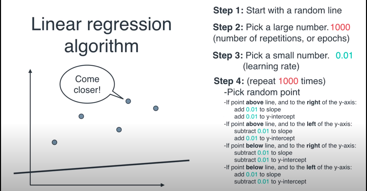
This is the screenshot I took from a video on linear regression made by Luis Serrano. He explained linear regression step by step (scratch version). The first step was to start with a random line.

The question is do we actually draw a random line, or instead do we perform some calculation like taking an average of y values and initially draw a line. Because if we take any random line it might not fall near any points at all. Maybe it will fall on the 3rd quadrant of the coordinate system where there are no points in this case.

Answer 1

NO

What we want to find are the parameters that result in the least amount of error, and OLS defines error as the squared differences between observed values $y_i$ and predicted values $\hat y_i$. Error often gets denoted by an $L$ for "loss".

$$ L(y, \hat y) = \sum_{i = 1}^N \bigg(y_i - \hat y_i\bigg)^2 $$

We have our regression model, $\hat y_i =\hat\beta_0 + \hat\beta_1x$, so the $\hat y$ is a function of $\hat\beta_0$ and $\hat\beta_1$.

$$ L(y, \hat\beta_0, \hat\beta_1) = \sum_{i = 1}^N \bigg(y_i - (\hat\beta_0 + \hat\beta_1x)\bigg)^2 $$

We want to find the $\hat\beta_0$ and $\hat\beta_1$ that minimize $L$.

What the video does is simulate pieces of the entire "loss function". For $\hat\beta_0 = 1$ and $\hat\beta_1 = 7$, you get a certain loss value. For $\hat\beta_0 = 1$ and $\hat\beta_1 = 8$, you get another loss value. One approach to finding the minimum is to pick random values until you find one that results in a loss value that seems low enough (or you're tired of waiting). Much of the deep learning work uses variations of this, with tricks like stochastic gradient descent to make the algorithm get (close to) the right answer in a short amount of time.

In OLS linear regression, however, calculus gives us a solution to the minimization problem, and we do not have to play such games.

$$\hat\beta_1=\frac{cov(x,y)}{var(x)}\\ \hat\beta_0=\bar y-\hat\beta_1\bar x$$

Answer 2

We, sort of, do something like this effectively, especially in Gradient descent algorithms. A random line is simply a set of random parameters $\beta_0,\beta_1$. The gradient descent algorithm has to start somewhere looking for the optimal parameters, and the random set of parameters is one place to start.

So, in a way, we do start with a line, though we don’t draw it. Also, the algorithm itself is not exactly the one presented, of course. The instructor was probably trying to explain it without the notion of a gradient, and it’s tough. So, I’d give him a pass on a sloppy attempt.

Answer 3

Sometimes it is more intuitive to show things graphically, mostly for beginners. You can do it this way, of course, but in practice this is not how it is done, as there is a closed form solution, as Frank Harrel mentioned in the comment. If you have a single independent variable, as in simple linear regression, $\hat y_i = \hat\beta_0 + \hat\beta_1x$, you solve it analytically, through the equations below:

$\hat\beta_1=\frac{cov(x,y)}{var(x)}$

and

$\hat\beta_0=\bar y-\beta_1\bar x$

By the way, it is possible that this question (Why is a regression coefficient covariance/variance?) is of your interest.

Answer 4

That example is definitely NOT the way linear regression is typically done, but I suppose it is an algorithm to find a regression line. As other answers have correctly stated, there is a closed form solution for finding the Least Squares Regression equation for a set of points.

That being said, what's being shown in the snippet is a method for algorithmically finding a line that gets close to the points by trial and error (i.e. iterations).

As a simple analogy to show the difference between a closed form solution and an algorithm: if I were to give you a mathematical equation, say $10 = 2x+4$, and asked you to solve for $x$, we know that you can solve this exactly using algebra.

$10 = 2x+4$

$\implies 2x=6$

$\implies x=3$ ** Exact solution **

Alternatively, an algorithmic approach to this could be used to solve this same equation by guessing a solution (e.g. start with a random guess: $x=0$) and systematically adjusting $x$ until your condition (statement of equality) is met, or approximately met.

$x = 0 \implies 10=4$ ** too low, adjust up **

$x = 1 \implies 10=6$ ** too low, adjust up **

$x = 2 \implies 10=8$ ** too low, adjust up **

$x = 3 \implies 10=10$ ** condition met, stop **

As this crude example shows, algorithms can sometimes approximate the answers returned by closed form solutions, but this isn't guaranteed to happen for all types of equations.

Personally, I don't find the snippet in the question to be pedagogically helpful to showing how regression lines work, and I think there are better examples of how algorithms can be used to find approximate solutions to mathematical equations.

Answer 5

This clearly looks like an attempt by an instructor to introduce some intuition behind linear regression and iterative optimisation to computer science students not familiar with derivatives or without a mathematical background in general.

If it was up to me I would do it in a slightly different way - start with some "goodness of fit" measure, then, since this is a simple linear regression with one covariate, perform a grid search over the intercept and slope, and calculate the selected goodness of fit measures for every point on a grid computationally using a loop.

This would give students some intuition and they would even feel being able to get an approximate answer themselves. After this step we then can mention that for some goodness of fit measures such problem can be solved precisely without the need to perform any iterations, but that doesn't change the goal or intuition behind looking for the best-fitting solution and minimising residuals.

Sticking with the iterative procedure, however, does require a starting point with a random line. This is similar to how some neural network optimisations start with initiation of random weights. Still, I feel, that calculating the goodness of fit to every subsequent iteration would help to clarify things further. Without it it might seem unclear why the line needs to move at all, and how is it getting any better by moving towards the points.

Answer 6

To be clear, there's a closed form solution for linear regression that is almost always used to find the fit, so there's no need for a "guess" to start with at all. This example is more of illustrative example of how Stochastic Algorithms work rather than how to best fit a linear regression model.

However, linear regression really is the exception to the rule in this case. For fitting most models, we do not have a closed form solution and we do need to start with an initial set of parameters and then iteratively improve them.

In such cases, it is often the case that choosing a good starting point, as you have suggested, will help the algorithm to converge faster. For some problems, choosing a good starting point is crucial for acceptable performance (both in terms of speed of convergence and probability that algorithm will converge to an acceptable answer), while for other model/algorithm combinations, the improvement may be so minor that it is not worth the extra effort to find a good starting values and initializing with random values is fine.

Answer 7

Some methods for robust regression, notably RANSAC (Random sample consensus) are actually built around fitting random lines. But this is, of course, far from what is happening here - I agree with those who say that

• it is a pedagogical tool
• the problem can be solved exactly (optimal least squares)
• it is reminiscent of the gradient descent

In the above mentioned robust methods one actually uses exact regression for fitting a line to a random subset of datapoints, thus diminishing the influence of the outliers (to which the exact solution to linear least squares regression is extremely sensitive).