I have a doubt about the Schoenfeld residuals that are used to check the Cox proportional hazard model.
The residuals formula is: $$\hat{r}_{ik}=c_i(x_{ik}-\hat{\bar{x}}_{w_ik})$$ $$\hat{\bar{x}}_{w_ik}=\frac{\sum_{j\in R(t_i)}x_{jk}e^{\vec{x}^{\intercal}_j\vec\beta}}{\sum_{j\in R(t_i)}e^{\vec{x}^{\intercal}_j\vec\beta}}$$
And, in theory, its plot should be on average on close to 0.
To test it I took the Weibull hazard function: $$h(t)=ba^{-b}t^{b-1}$$ And rewrote it as: $$h(t)=be^{-b\cdot log(a)}t^{b-1}$$ The Cox proportional hazard model is: $$h(t,\vec{x},\vec{\beta})=h_0(t)\cdot e^{\vec{\beta}^{\intercal}\vec{x}}$$ That, in this case, becomes: $$h_0(t)=bt^{b-1}$$ $$\vec\beta=-b$$ $$\vec{x}=log(a)$$
I then tried simulating with MATLAB 1000 uncensored events, randomly split with $a=10$ and $a=20$ and having $b=2$.
I hypothesized my Cox proportional hazard model were able to correctly identify $h_0(t)=bt^{b-1}$ and $\vec\beta=-b$ and computed the theoretical Schoenfeld residuals:
$$\hat{r}_{ik}=log(a_i)-\hat{\bar{x}}_{w_i}$$
$$\hat{\bar{x}}_{w_i}=\frac{\sum_{j\in R(t_i)}log(a_j)e^{-b\cdot log(a_j)}}{\sum_{j\in R(t_i)}e^{-b\cdot log(a_j)}}$$
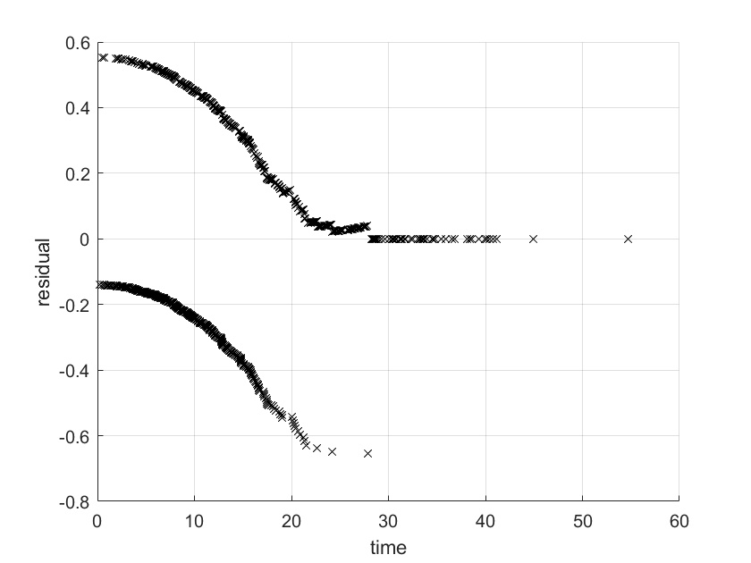
The result was this:
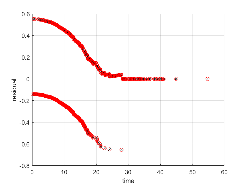
 I also tried fitting a Cox proportional hazard model and computing the Schoenfeld residuals automatically (red circles):
 The both cases average residuals are not close to 0 at all. I am not sure what I am missing.
I took the Schoenfeld residual formula from:
Applied Survival Analysis: Regression Modelling of Time-to-Event Data, 2nd Edition

survival::plot.cox.zphfunction in R defaults to a spline with 4 degrees of freedom $\endgroup$