185
$\begingroup$

On the Wikipedia page about naive Bayes classifiers, there is this line:

$p(\mathrm{height}|\mathrm{male}) = 1.5789$ (A probability distribution over 1 is OK. It is the area under the bell curve that is equal to 1.)

How can a value $>1$ be OK? I thought all probability values were expressed in the range $0 \leq p \leq 1$. Furthermore, given that it is possible to have such a value, how is that value obtained in the example shown on the page?

$\endgroup$
7
  • 5
    $\begingroup$ When I saw that i thought it might be the height of the probability density function which can be any positive number as long as when it is integrated over any interval, the integral is less than or equal to 1. Wikipedia should correct that entry. $\endgroup$ Commented May 5, 2012 at 2:05
  • 19
    $\begingroup$ Because this might help future readers, I offer a geometric translation of the general part of this question: "How can a shape whose area does not exceed $1$ possibly extend more than $1$ in any direction?" Specifically, the shape is that part of the upper half plane bounded above by the graph of the PDF and the direction in question is vertical. In the geometric setting (shorn of the probability interpretation) it's easy to think of examples, such as a rectangle of base no greater than $1/2$ and height $2$. $\endgroup$
    – whuber
    Commented May 29, 2012 at 18:17
  • 2
    $\begingroup$ the Wikipedia article now uses lowercase p for probability density and uppercase P for probability $\endgroup$
    – Aprillion
    Commented Apr 17, 2013 at 10:00
  • 4
    $\begingroup$ Worth noting that a Cumulative Distribution Function (the integral of the PDF) can't go above 1. The CDF is a lot more intuitive to use in many cases. $\endgroup$
    – naught101
    Commented Mar 27, 2019 at 1:23
  • 1
    $\begingroup$ @HeyJude: Dirac delta function takes an infinite value at one point but the area under the curve is 1. $\endgroup$
    – Joshua
    Commented Dec 6, 2023 at 16:04

6 Answers 6

209
$\begingroup$

That Wiki page is abusing language by referring to this number as a probability. You are correct that it is not. It is actually a probability per foot. Specifically, the value of 1.5789 (for a height of 6 feet) implies that the probability of a height between, say, 5.99 and 6.01 feet is close to the following unitless value:

$$1.5789\, [1/\text{foot}] \times (6.01 - 5.99)\, [\text{feet}] = 0.0316$$

This value must not exceed 1, as you know. (The small range of heights (0.02 in this example) is a crucial part of the probability apparatus. It is the "differential" of height, which I will abbreviate $d(\text{height})$.) Probabilities per unit of something are called densities by analogy to other densities, like mass per unit volume.

Bona fide probability densities can have arbitrarily large values, even infinite ones.
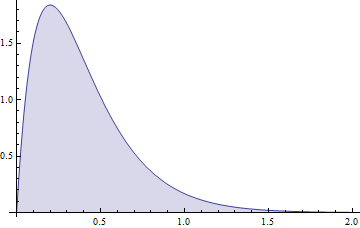
Gamma distribution

This example shows the probability density function for a Gamma distribution (with shape parameter of $3/2$ and scale of $1/5$). Because most of the density is less than $1$, the curve has to rise higher than $1$ in order to have a total area of $1$ as required for all probability distributions.
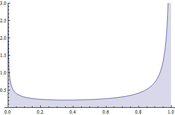
Beta distribution

This density (for a beta distribution with parameters $1/2, 1/10$) becomes infinite at $0$ and at $1$. The total area still is finite (and equals $1$)!


The value of 1.5789 /foot is obtained in that example by estimating that the heights of males have a normal distribution with mean 5.855 feet and variance 3.50e-2 square feet. (This can be found in a previous table.) The square root of that variance is the standard deviation, 0.18717 feet. We re-express 6 feet as the number of SDs from the mean:

$$z = (6 - 5.855) / 0.18717 = 0.7747$$

The division by the standard deviation produces a relation

$$dz = d(\text{height})/0.18717$$

The Normal probability density, by definition, equals

$$\frac{1}{\sqrt{2 \pi}}\exp(-z^2/2)dz = 0.29544\ d(\text{height}) / 0.18717 = 1.5789\ d(\text{height}).$$

(Actually, I cheated: I simply asked Excel to compute NORMDIST(6, 5.855, 0.18717, FALSE). But then I really did check it against the formula, just to be sure.) When we strip the essential differential $d(\text{height})$ from the formula only the number $1.5789$ remains, like the Cheshire Cat's smile. We, the readers, need to understand that the number has to be multiplied by a small difference in heights in order to produce a probability.

$\endgroup$
12
  • 2
    $\begingroup$ I note that the example given on that wiki page uses probability densities in lieu of actual probabilities for the calculation of posteriors, presumably because the per unit aspect is not necessary for comparative purposes if the units being compared are the same. Extending this, if one doesn't want to assume normality but instead one has empirical data from which density can be estimated, e.g. a kernel density estimate, would it be valid to use a reading at a given value on the x-axis from this kde as input to calculating posteriors in a naive bayes classifier, assuming equal per units? $\endgroup$ Commented Nov 7, 2010 at 17:08
  • 3
    $\begingroup$ @babelproofreader I believe the posteriors are Bayesian updates, via the training data, of priors. It's unclear how a kde could be construed similarly, but I'm no expert in this area. Your question is interesting enough that you might consider posting it separately. $\endgroup$
    – whuber
    Commented Nov 7, 2010 at 17:23
  • 1
    $\begingroup$ How do you determine what is a good differential? What If you had picked a differential of 1 instead? the probability would then be larger than 1? Sorry for my confusion here. Can you explain? $\endgroup$
    – fiacobelli
    Commented Oct 10, 2014 at 18:34
  • 5
    $\begingroup$ @tree The area of a triangle is one half the product of the length of its base and its height. $\endgroup$
    – whuber
    Commented Jan 22, 2015 at 16:15
  • 2
    $\begingroup$ @user929304 You may refer to any theoretical textbook that appeals to you: this is part of the fundamentals of probability and statistics. This particular concept of probability density is nicely discussed in the better introductory textbooks, such as Freedman, Pisani, & Purves. $\endgroup$
    – whuber
    Commented Jun 24, 2016 at 14:03
52
$\begingroup$

This is a common mistake from not understanding the difference between probability mass functions, where the variable is discrete, and probability density functions, where the variable is continuous. See What is a probability distribution:

continuous probability functions are defined for an infinite number of points over a continuous interval, the probability at a single point is always zero. Probabilities are measured over intervals, not single points. That is, the area under the curve between two distinct points defines the probability for that interval. This means that the height of the probability function can in fact be greater than one. The property that the integral must equal one is equivalent to the property for discrete distributions that the sum of all the probabilities must equal one.

$\endgroup$
3
  • 17
    $\begingroup$ The NIST is usually authoritative, but here it is technically incorrect (and ungrammatical to boot): having a probability defined at "an infinite number of points" does not imply the "probability at a single point is always zero." Of course they're just dodging a distraction about infinite cardinalities, but the reasoning here is misleading. It would be better for them just to omit the first sentence in the quotation. $\endgroup$
    – whuber
    Commented Nov 5, 2010 at 15:20
  • 1
    $\begingroup$ Assuming a hypothetical continuous PDF, the probability at a single point is, generally, infinitely small (think limits in calculus). If the probably was "always zero" then, by definition, no such result would be possible. $\endgroup$ Commented Oct 17, 2019 at 5:07
  • 1
    $\begingroup$ Many highly competent writers are happy to write about density with respect to counting measure. In effect non-mathematicians (I am one) are often told that probability mass and probability density are quite different ideas, which they should never confuse, while mathematicians should know better, depending on how much measure theory they know. $\endgroup$
    – Nick Cox
    Commented Jun 8, 2022 at 10:18
29
$\begingroup$

I think that a continuous uniform distribution over an interval $[a,b]$ provides a straightforward example for this question: In a continuous uniform distribution the density in each point is the same at each point (uniform distribution). Moreover, because the area below the rectangle must be one (just as the area below the normal curve must be one) that density value must be $1/(b-a)$ because any rectangle with base $b-a$ and area $1$ must have height $1/(b-a)$ .

So the value for the uniform density on the interval $[0,0.5]$ is $1/(0.5-0)=2$, on the interval $[0,0.1]$ it is $10$, ...

$\endgroup$
0
4
$\begingroup$

I don't know whether the Wikipedia article has been edited subsequent to the initial posts in this thread, but it now says "Note that a value greater than 1 is OK here – it is a probability density rather than a probability, because height is a continuous variable.", and at least in this immediate context, P is used for probability and p is used for probability density. Yes, very sloppy since the article uses p in some places to mean probability, and in other places as probability density.

Back to the original question "Can a probability distribution value exceeding 1 be OK?" No, but I've seen it done (see my last paragraph below).

Here's how to interpret a probability > 1. First of all, note that people can and do give a 150% effort, as we often hear in sports and sometimes work https://www.youtube.com/watch?v=br_vSdAOHQQ . If you're sure something will happen, that's a probability of 1. A probability of 1.5 could be interpreted as you're 150% sure the event will happen - kind of like giving a 150% effort.

And if you can have a probability > 1, I suppose you can have a probability < 0. Negative probabilities can be interpreted as follows. A probability of 0.001 means there's almost no chance of the event happening. Probability = 0 means "no way". A negative probability, such as -1.2, corresponds to "You gots to be kidding".

When I was a wee lad just out of school 3 decades ago, I witnessed an event more astounding than breaking the sound barrier in aviation, namely, breaking the unity barrier in probability. An analyst with a Ph.D. in Physics had spent 2 years full-time (probably giving 150%) developing a model for calculating the probability of detecting object X, at the end of which his model and analysis successfully completed peer review by several scientists and engineers closely affiliated to the U.S. government. I won't tell you what object X is, but object X, and the probability of detecting it, was and still is of considerable interest to the U.S. government. The model included a formula for $P_y$ = Prob(event y happens). $P_y$ and some other terms all combined into the final formula, which was Prob(object X is detected). Indeed, computed values of Prob(object X is detected) were within the range of [0,1], as is "traditional" in probability in the Kolmogorov tradition. $P_y$ in its original form was always in [0,1] and involved "garden-variety" transcendental functions which were available in standard Fortran or any scientific calculator. However, for a reason known only but to the analyst and God (perhaps because he had seen it done in his Physics classes and books, but did not know that he was shown the few cases where it works, not the many more where it does not, and this guy's name and scientific/mathematical judgment did not happen to be that of Dirac), he chose to take a two term Taylor expansion of $P_y$ (and ignore the remainder term), which will henceforth be referred to as $P_y$. It was this two term Taylor expansion of $P_y$ which was inserted into the final expression for Prob(object X is detected). What he did not realize, until I pointed it out to him, was that $P_y$ was equal to approximately 1.2 using his base case values for all parameters. Indeed it was possible for $P_y$ to go up to about 1.8. And that's how the unity barrier was broken in probability. But the guy didn't know he had accomplished this pioneering feat until I pointed it out to him, having just performed quick calculations on a battery-powered credit card size Casio scientific calculator in a darkened conference room (couldn't have done it with a solar-powered calculator). That would be kind of like Chuck Yeager going out for a Sunday spin in his plane, and only being informed months later that he had broken the sound barrier.

$\endgroup$
2
3
$\begingroup$

When random variable $X$ is continuous and its probability density function is $f(x)$, $f(x)dx$ is a probability, but $f(x)$ is not a probability and can be larger than one. The reported $f(\mbox{height}|\mbox{male})$ is not a probability, but $f(\mbox{height}|\mbox{male})d\mbox{height}$ is.

In other words, for a continuous random variable $X$, $P(X\in[x,x+dx))=f(x)dx$, $P(X\in[a,b])=\int_{a}^{b}f(x)dx$, and $P(X = x)=P(X \in [x,x])=0$. The same goes for conditional probabilities.

$\endgroup$
1
  • $\begingroup$ so it's like...for a continuous random variable with pdf $f$, the rule is $f \ge 0$ but no one ever said $1 \ge f$ ? $\endgroup$
    – BCLC
    Commented Aug 19, 2021 at 23:48
-1
$\begingroup$

The point value at a particular parameter value of a probability density plot would be a likelihood, right? If so, then the statement might be corrected by simply changing P(height|male) to L(height|male).

$\endgroup$

Not the answer you're looking for? Browse other questions tagged or ask your own question.