Detecting peaks in noisy quasi-periodic time series

Question

I have the following acceleration data taken from my phone when rowing

The negative peak is the point at which the oars go in the water. I would like to be able to identify this peak in real time when rowing.

Given the data is roughly periodic - with frequency between 0.1 and 1 times per second - and has a characteristic shape. What would be the best way to detect these peaks in real time?

data here for anyone interested: acceleration data

Answer 1

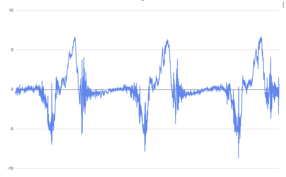
One of the simplest ways that is likely to work follows a "smooth, detect, check" workflow.

1. Smooth the data to suppress noise. A running convolution with an extremely smooth kernel is a good idea because it will produce smooth derivatives, too. I use a Gaussian.

2. Detect the troughs. To do this reliably you want (a) the smoothed value to be relatively low and (b) to be genuinely in a trough rather than a local dip. To this end, maintain (1) a smoothed version of the typical amplitude and (2) an estimate of the second derivative of the signal.

3. Check the results by looking around in a small temporal neighborhood of the apparent trough locations. Often, a trough will result in a short burst of detections. You may locate the trough with the first, the last, or the middle time in that burst if you like.

There are some parameters to tune. The most important is the smoothing bandwidth: too small, and it will not reduce the noise and create spurious detections; too large, and the times of the troughs will be imprecise (and it will take too long to detect them: the time lapse needed for a kernel smooth equals its bandwidth).

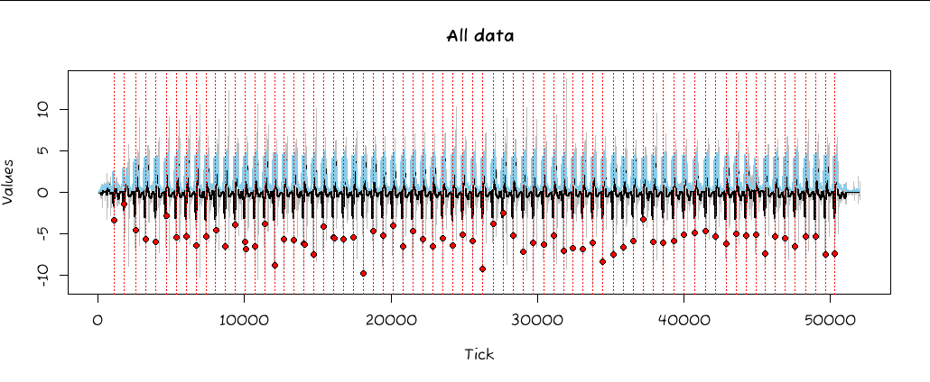
Here is an automatically generated solution.

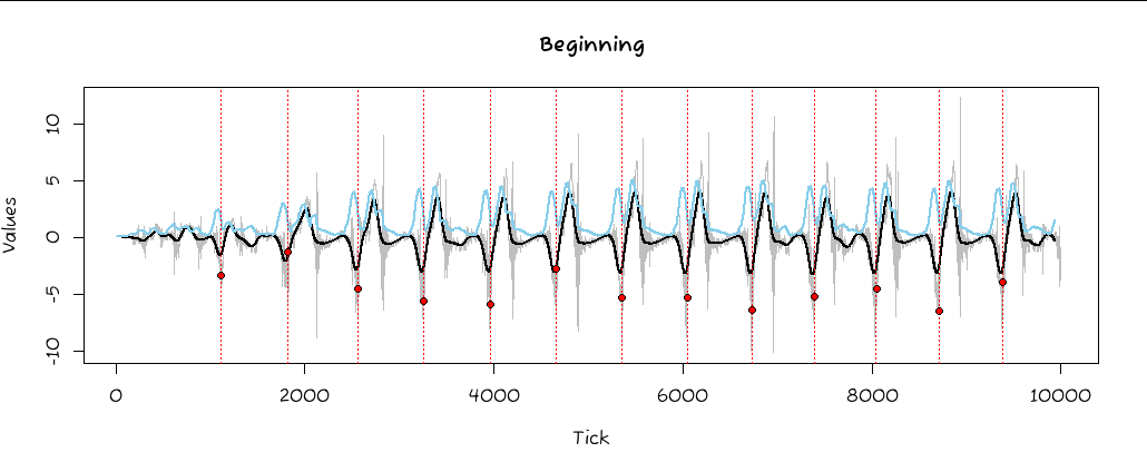
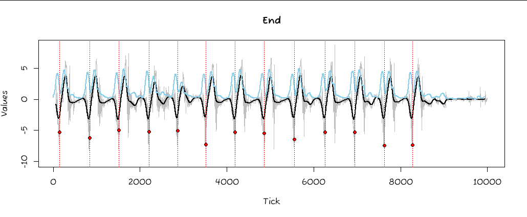
The faint gray trace is the original data; the black version is its smooth with a bandwidth of 64 ticks (about one-tenth of a cycle); the light blue plots the second derivative; and the red dots locate the estimated troughs. Dashed red lines are drawn through those points to show how regularly they appear.

Some details at the beginning and end of the procedure show more clearly what is going on.

The estimated locations of the troughs look very accurate, especially once the amplitude reaches its quasi steady state after time 2000.

At the end, this procedure gracefully shuts down and does not detect spurious troughs.

I wrote this R code to emphasize the sequential nature of this detection process. (It would be more efficient to collect the entire dataset and use the Fast Fourier Transform for the smoothing if you don't need real-time detection.)

#
# Initialize an object to maintain information about a narrow time window.
# `W` is the most recent window of data while `A` holds their squared amplitudes
# (within, potentially, a window of different length).
#
initialize <- function(h) {
  k <- dnorm(seq(-2, 2, length.out = 2*h + 1)); k <- k / sum(k)
  u <- rep(1/h, h)
  list(i = -h, y = NA, a = NA, h = h, K = k, U = u, W = rep(NA, 0), A = rep(0, 0))
}
#
# Process the next datum, returning the updated object.
# The caller will use the update for trough detection.
#
update <- function(x, obj) {
  within(obj, {
    if (length(W) >= length(K)) W <- W[-1]
    if (length(A) >= length(U)) A <- A[-1]
    W <- c(W, x)
    A <- c(A, x^2)
    if (length(W) >= length(K)) y <- sum(K * W) else y <- NA
    if (length(A) >= length(U)) a <- sqrt(sum(U * A)) else a <- NA
    i <- i + 1
  })
}
#
# Read the sample data.
#
X <- read.csv("C:/Users/whube/Downloads/acceleration.txt", header = FALSE)$V1
# X <- X[(length(X) - 1e4 + 1):length(X)]
# X <- X[1:1e4]
n <- length(X)
#
# Process the data sequentially.
#
initialize(2^6) -> obj
Y <- matrix(rep(NA, 4*n), 4, dimnames = list(c("i", "y", "a", "trough"), NULL))
for (i in 1:n) {
  obj <- update(X[i], obj)
  
  # Detect troughs.  Store the updated values for later plotting.
  Y[, i] <- with(obj, {
    c(i, y, a, y <= -a/3 & a > 2)
    })
}
#
# Plot the results.
#
plot(obj$h:n, X[obj$h:n], type = "l", col = gray(0.75), 
     main = "End", family = "Informal",
     xlab = "Tick", ylab = "Values")
lines(seq_len(n) - obj$h, Y["y", ], col = "Black", lwd = 2)
lines(seq_len(n) - length(obj$U), Y["a",], col = "skyblue", lwd = 2)
#
# Plot the trough locations.
# This uses a little post-processing to merge short bursts of troughs into
# single time points.  This typically takes only a handful of ticks, 
# maintaining the real-time quality of the algorithm.
#
v <-  which(Y["trough", ]==1) - obj$h
j <- which(diff(c(v, Inf)) > 1)
abline(v = v[j-1], lty = 3, col = "Red")

z <- apply(rbind(v[j-1], v[j]), 2, function(k) min(X[k[1]:k[2]]))
k <- apply(rbind(v[j-1], v[j]), 2, function(k) which.min(Y["y", k[1]:k[2]]) + k[1]-1)
points(k, z, pch = 21, bg = "Red")